Step by Step :Understanding Linear Regression in Data Analytics
Linear regression is a fundamental statistical technique widely used in data analytics to model the relationship between a dependent variable and one or more independent variables. It serves as a valuable tool for predicting outcomes and understanding the underlying patterns within datasets. In this blog, we’ll delve into the intricacies of linear regression, exploring its concepts, applications, and practical considerations.
Table of Contents
ToggleWhat is Linear Regression?
Linear regression is a statistical method used in data analysis and machine learning to model the relationship between a dependent variable and one or more independent variables. The goal is to find the best-fitting linear equation that describes the relationship between the variables. In essence, linear regression helps us understand how changes in one variable are associated with changes in another.
The fundamental assumption behind linear regression is that there exists a linear relationship between the dependent variable (the one we are trying to predict) and the independent variable(s) (the ones used for prediction). This relationship is represented by a straight line equation:
Y=mX+b
where:
- Y is the dependent variable.
- X is the independent variable.
- m is the slope of the line, indicating the change in
- Y for a unit change in X.
- b is the y-intercept, representing the value of
- Y when X is 0.
Types of Linear Regression:
Simple Linear Regression:
In simple linear regression, there is only one independent variable predicting the dependent variable. The equation takes the form
Y=b0+b1X
where
b0 is the y-intercept, b1 is the slope, and X is the independent variable.
Multiple Linear Regression:
This involves more than one independent variable and one dependent variable. The equation for multiple linear regression is:
where:
Y is the dependent variable
X1, X2, …, Xp are the independent variables
β0 is the intercept
β1, β2, …, βn are the slopes
Simple Linear Regression with Python
import pandas as pd


# Load the dataset from CSV
excel_sheet='study hours'
df=pd.read_excel('E:\constructor\stack chart.xlsx',excel_sheet)
df
import numpy as np
from sklearn.linear_model import LinearRegression
import matplotlib.pyplot as plt
# Extract the features (X) and target variable (y)
X = df[['Hours Studied']]
y = df['Exam Scores']

# Create a linear regression model
model = LinearRegression()

# Fit the model to the data
model.fit(X, y)

# Make predictions based on the model
predictions = model.predict(X)

# Visualize the results
plt.scatter(X, y, label='Actual Data')
plt.plot(X, predictions, color='red', label='Linear Regression Line')
plt.xlabel('Hours Studied')
plt.ylabel('Exam Scores')
plt.title('Simple Linear Regression in Python')
plt.legend()
plt.show()

# Print the equation of the line
slope = model.coef_[0]
intercept = model.intercept_
print(f"Linear Regression Equation: y = {slope:.2f} * x + {intercept:.2f}") 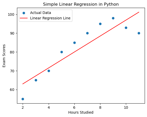
the code step by step to understand each part:
import pandas as pd
import numpy as np
from sklearn.linear_model import LinearRegression
import matplotlib.pyplot as plt
Import Libraries:
- import pandas as pd: Imports the Pandas library, which is used for data manipulation and analysis.
- import numpy as np: Imports the NumPy library, which provides support for large, multi-dimensional arrays and matrices, along with mathematical functions.
- from sklearn.linear_model import LinearRegression: Imports the LinearRegression class from scikit-learn, a machine learning library in Python.
- import matplotlib.pyplot as plt: Imports the pyplot module from the Matplotlib library, which is used for creating visualizations.
# Load the dataset from CSV
df = pd.read_csv("dataset.csv")
Load the Dataset:
pd.read_csv(“dataset.csv”): Reads the dataset from a CSV file named “dataset.csv” and stores it in a Pandas DataFrame named df. Make sure to replace “dataset.csv” with the actual path to your dataset.
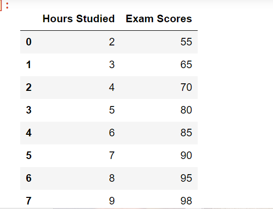
# Extract the features (X) and target variable (y) with explicit column names
X = df[['Hours Studied']]
y = df['Exam Scores']
Prepare Features and Target Variable:
- X = df[[‘Hours Studied’]]: Extracts the feature variable (independent variable) ‘Hours Studied’ as a DataFrame.
- y = df[‘Exam Scores’]: Extracts the target variable (dependent variable) ‘Exam Scores’ as a Series.
# Create a linear regression model
model = LinearRegression()
Create Linear Regression Model: model = LinearRegression(): Initializes an instance of the LinearRegression model from scikit-learn.
# Fit the model to the data
model.fit(X, y)
Fit the Model:
- model.fit(X, y): Fits the linear regression model to the training data, where X is the feature variable, and y is the target variable.
# Make predictions based on the model
predictions = model.predict(X)
Make Predictions: predictions = model.predict(X): Uses the trained model to make predictions on the feature variable X. Predicted values are stored in the predictions variable.
# Visualize the results
plt.scatter(X, y, label='Actual Data')
plt.plot(X, predictions, color='red', label='Linear Regression Line')
plt.xlabel('Hours Studied')
plt.ylabel('Exam Scores')
plt.title('Simple Linear Regression in Python')
plt.legend()
plt.show()
Visualize the Results:
Uses Matplotlib to create a scatter plot of the actual data points (X and y) and overlays the linear regression line. This helps visualize how well the model fits the data.
# Print the equation of the line
slope = model.coef_[0]
intercept = model.intercept_
print(f"Linear Regression Equation: y = {slope:.2f} * x + {intercept:.2f}")
Print the Equation of the Line:
Uses the coefficients and intercept obtained from the trained model to print the equation of the fitted line. make new prediction
# Make a new prediction
new_hours_studied = np.array([[12]])  # Replace this with the hours you want to predict
predicted_exam_scores = model.predict(new_hours_studied)

# Print the predicted exam scores
print(f"Predicted Exam Scores: {predicted_exam_scores[0]:.2f}")
Make a New Prediction:
Uses the trained model to make a prediction for a new set of hours studied (in this case, 12 hours). The result is printed to the console.
This script demonstrates the entire workflow of loading data, creating a simple linear regression model, fitting it to the data, visualizing the results, and making predictions. Adjustments can be made based on the specific dataset and requirements.