Machine learning algorithms for data analytics

21Mar, 2024

Mastering Machine Learning: The Top 10 Algorithms You Need to Know

In today’s data-driven world, machine learning has become an indispensable tool for extracting valuable insights from vast amounts of data. However, for beginners entering the realm of machine learning, the plethora of algorithms available can seem overwhelming. Understanding the fundamental algorithms is crucial for building a strong foundation in this field.

Linear Regression

Linear regression is a statistical method used in machine learning to predict continuous outcomes or values based on input features. Let’s break down how linear regression works in simple steps:

Understanding the Concept:

Imagine you have some data where you know the input (like the size of a house) and the output (like the price of the house). Linear regression helps us find the relationship between these inputs and outputs.

Plotting the Data:

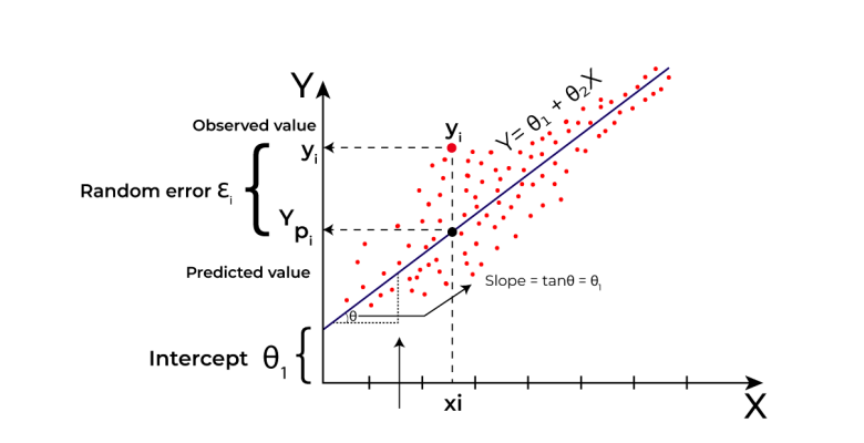
We start by plotting our data points on a graph, with the input values on the x-axis and the corresponding output values on the y-axis. This gives us a scatterplot of our data points.

Drawing a Line:

Linear regression finds the best-fitting line through the data points. This line represents the relationship between the input and output variables. The goal is to find the line that minimizes the difference between the actual data points and the predicted values on the line.

The Equation of the Line:

The equation of the line in linear regression is represented as:
Y = mX + c
Y represents the predicted output value.
X represents the input feature.
m is the slope of the line, which represents how much the output value changes for a one-unit change in the input feature.
c is the y-intercept, which represents the value of Y when X is 0.

Finding the Best-Fitting Line:

Linear regression uses a method called least squares to find the best-fitting line. It calculates the sum of the squares of the vertical distances between the data points and the line. The line that minimizes this sum is considered the best-fitting line.

Making Predictions:

Once we have the equation of the best-fitting line, we can use it to make predictions. Given a new input value, we can plug it into the equation to predict the corresponding output value.

Evaluating the Model:

Finally, we evaluate the performance of our linear regression model by comparing the predicted values to the actual values in our dataset. Common evaluation metrics include mean squared error (MSE) or R-squared.

Extensions to Complex Models:

While linear regression is simple and easy to understand, it forms the basis for more complex regression techniques like polynomial regression, ridge regression, or lasso regression, which can handle more intricate relationships between variables.

In summary, linear regression is a powerful tool for predicting continuous values based on input features. By finding the best-fitting line through the data points, it allows us to understand and quantify relationships between variables in our dataset.

Logistic regression

Logistic regression is a fundamental algorithm in machine learning, primarily used for binary classification problems. Let’s delve into how logistic regression works step by step, explained in simple terms:

Binary Classification:

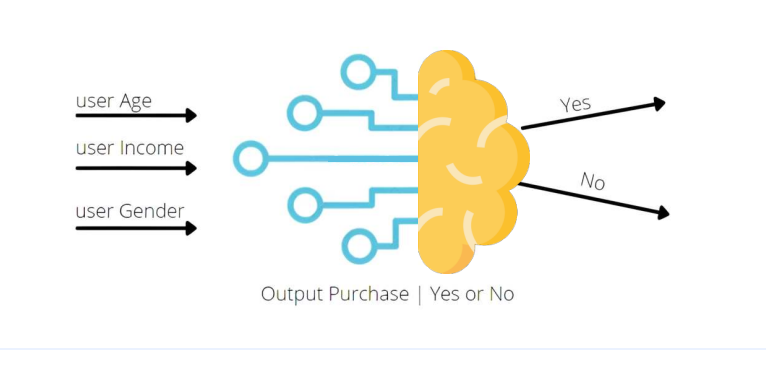
Binary classification means we have two possible outcomes for our prediction: yes or no, 0 or 1, true or false. For example, predicting whether an email is spam or not spam, whether a transaction is fraudulent or legitimate, etc.

Understanding Probability:

Logistic regression predicts the probability of one of the two outcomes occurring. Instead of directly predicting 0 or 1, it predicts a probability value between 0 and 1.

Sigmoid Function:

Logistic regression uses a special function called the sigmoid function (also known as the logistic function). This function maps any real-valued number to a value between 0 and 1. The formula for the sigmoid function is:

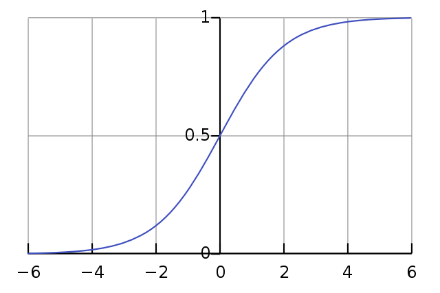
Here, “x” represents the input value, and “σ(x)” represents the output, which is the probability of the event occurring.

Linear Equation:

Like linear regression, logistic regression also has an equation, but it’s slightly different. Instead of a straight line, logistic regression uses a line that’s curved due to the sigmoid function. The equation looks like this:
Logistic Regression Equation
Here, “z” represents the linear combination of input features and their respective coefficients, just like in linear regression.

Probability Interpretation:

Once we have the output from the sigmoid function (which is a probability), we can interpret it as follows: if the probability is closer to 0, it means the event is less likely to occur, and if it’s closer to 1, it means the event is more likely to occur.

Decision Boundary:

Logistic regression separates the input space into two regions using a decision boundary. If the probability is above a certain threshold (usually 0.5), we predict one class (e.g., 1), and if it’s below the threshold, we predict the other class (e.g., 0).

Training the Model:

During training, logistic regression adjusts its coefficients to minimize the difference between the predicted probabilities and the actual outcomes in the training data. It does this using optimization algorithms like gradient descent.

Evaluation:

To evaluate the logistic regression model, we use metrics like accuracy, precision, recall, F1 score, etc., depending on the specific problem and requirements.

In summary, logistic regression is a powerful algorithm for binary classification problems, predicting the probability of an event occurring and making decisions based on that probability.

Decision Trees

Decision trees are versatile and intuitive models used in machine learning for both classification and regression tasks. Let’s explore how decision trees work in a step-by-step manner, emphasizing their simplicity and interpretability:

Intuitive Representation:

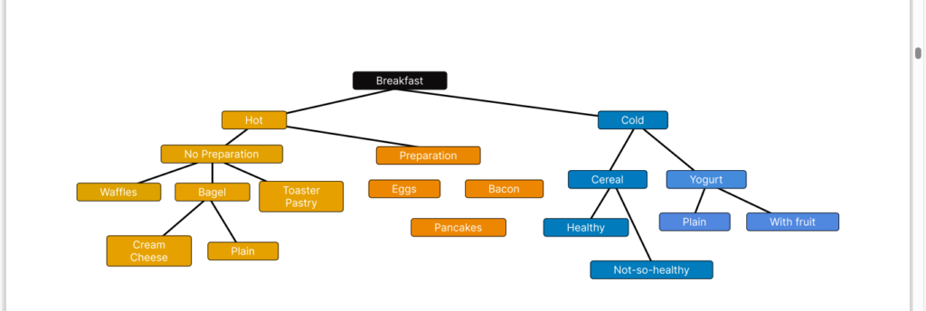
Decision trees mimic the human decision-making process by breaking down complex decision-making into a series of simple questions. Each node in the tree represents a decision based on a feature, and each branch represents the possible outcomes of that decision.

Feature Space Partitioning:

Decision trees partition the feature space into regions by recursively splitting the data based on feature values. At each step, the algorithm selects the feature that best separates the data into distinct classes or groups.

Splitting Criteria:

The decision tree algorithm evaluates different splitting criteria to determine the best feature and threshold for splitting the data at each node. Common splitting criteria include Gini impurity for classification tasks and mean squared error for regression tasks.

Building the Tree:

The decision tree algorithm continues to split the data recursively until certain stopping criteria are met, such as reaching a maximum depth, minimum number of samples per leaf node, or no further improvement in purity or error reduction.

Leaf Nodes:

Once the data is partitioned into homogeneous subsets or reaches the stopping criteria, the algorithm assigns a class label (for classification) or predicts a continuous value (for regression) at the leaf nodes of the tree.

Interpretability:

One of the key advantages of decision trees is their interpretability. The decision rules at each node can be easily understood and visualized, making it straightforward to interpret the model’s predictions and understand the factors influencing them.

Handling Categorical and Numerical Features:

Decision trees can handle both categorical and numerical features without requiring feature scaling or one-hot encoding. They automatically select the best split points for numerical features and perform multiway splits for categorical features.

Handling Missing Values:

Decision trees can handle missing values in the dataset by selecting the best split based on the available data, allowing for robust performance in real-world datasets with incomplete information.

Ensemble Methods:

Decision trees can be combined into ensemble methods such as random forests and gradient boosting, further improving predictive performance and generalization while retaining interpretability to some extent.

In summary, decision trees are powerful and intuitive models that partition the feature space into regions, making them suitable for both classification and regression tasks. Their simplicity, interpretability, and ability to handle a variety of data types make them a popular choice in many machine learning applications.

Random Forest

Random Forest is a robust and versatile ensemble learning technique that leverages the power of multiple decision trees to enhance predictive accuracy and mitigate overfitting. Here’s an explanation of how Random Forest works:

Ensemble Learning:

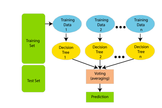
Random Forest belongs to the family of ensemble learning algorithms. Ensemble learning combines the predictions of multiple individual models to produce a more accurate and robust final prediction.

Construction of Decision Trees:

Random Forest constructs a predefined number of decision trees, typically referred to as “trees” or “estimators”. Each decision tree is built using a random subset of the training data and a random subset of the features.

Randomness and Diversity:

The randomness introduced in building individual trees helps to create diversity among them. Each tree may focus on different subsets of features and data instances, capturing different aspects of the underlying patterns in the data.

Bagging (Bootstrap Aggregating):

Random Forest employs a technique called bagging, where each decision tree is trained on a bootstrap sample of the training data. Bootstrap sampling involves randomly selecting data points with replacement, allowing some instances to be selected multiple times and others not at all.

Feature Randomness:

In addition to using bootstrap samples, Random Forest also introduces randomness in feature selection for each split of the decision tree. Instead of considering all features at each split, a random subset of features is considered, further enhancing diversity among the trees.

Combining Predictions:

Once all the decision trees are trained, Random Forest combines their predictions to make the final prediction. For classification tasks, it typically uses a majority voting scheme, where the class predicted by the majority of trees is chosen. For regression tasks, it averages the predictions made by individual trees.

Advantages of Random Forest:

Random Forest is highly resistant to overfitting due to the averaging effect of multiple trees.
It performs well on a wide range of datasets and can handle high-dimensional feature spaces.
Random Forest provides estimates of feature importance, allowing insights into the relative importance of different features in making predictions.

Hyperparameters:

Random Forest has several hyperparameters that can be tuned to optimize performance, such as the number of trees, maximum depth of trees, and the number of features considered at each split.
In summary, Random Forest is a powerful ensemble learning technique that combines the predictions of multiple decision trees to achieve higher accuracy and reduce the risk of overfitting, making it a popular choice for various machine learning tasks.

Support Vector Machines (SVM)

Support Vector Machines (SVM) is a versatile machine learning algorithm used for both classification and regression tasks. Let’s break down how SVM works:

Classification and Regression:

SVM can be used for both classification and regression tasks. In classification, SVM aims to classify data points into different categories, while in regression, it predicts continuous outcomes.

Hyperplane:

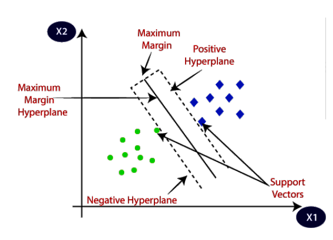
At the core of SVM is the concept of a hyperplane, which is a decision boundary that separates different classes in the feature space. For a binary classification problem, the hyperplane is a line in two dimensions, a plane in three dimensions, and a hyperplane in higher dimensions.

Maximizing Margin:

SVM finds the hyperplane that maximizes the margin, which is the distance between the hyperplane and the closest data points (support vectors) from each class. Maximizing the margin helps SVM generalize well to unseen data and improves its performance.

Support Vectors:

Support vectors are the data points that lie closest to the hyperplane and influence its position. These points are crucial in defining the decision boundary and are used to maximize the margin.

Kernel Trick:

SVM can efficiently handle non-linearly separable data by mapping the input features into a higher-dimensional space using a kernel function. The kernel function computes the dot product between feature vectors in the higher-dimensional space without explicitly transforming them. Common kernel functions include linear, polynomial, and radial basis function (RBF) kernels.

C Parameter:

SVM has a regularization parameter, often denoted as C, that controls the trade-off between maximizing the margin and minimizing the classification error. A smaller value of C allows for a wider margin but may lead to misclassification of some data points, while a larger value of C reduces the margin to classify more data points correctly.

Soft Margin SVM:

In cases where the data is not linearly separable or contains outliers, SVM uses a soft margin approach. Soft margin SVM allows for some misclassification errors by introducing slack variables, which penalize data points that fall on the wrong side of the margin or hyperplane.

Regression with SVM:

In regression tasks, SVM aims to find a hyperplane that best fits the data points while minimizing the error between the predicted and actual values. The epsilon-insensitive loss function is used to define a margin of tolerance around the fitted hyperplane.

In summary, Support Vector Machines (SVM) is a powerful algorithm for both classification and regression tasks. By finding the hyperplane that best separates different classes in the feature space, SVM achieves effective decision boundaries and generalization performance.

K-Nearest Neighbors (KNN)

K-Nearest Neighbors (KNN) is a straightforward yet powerful algorithm used for classification and regression tasks. Let’s explore how KNN works in simple terms:

Nearest Neighbor Classification:

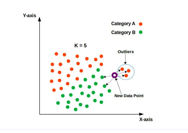
In KNN, the classification of a data point is determined by the majority class among its k nearest neighbors in the feature space.

Distance Metric:

KNN calculates the distance between data points using a chosen distance metric, commonly the Euclidean distance. Other distance metrics such as Manhattan distance or cosine similarity can also be used depending on the nature of the data.

Choosing ‘k’:

The value of ‘k’ represents the number of nearest neighbors to consider when making a prediction. It is an important hyperparameter in KNN and can significantly impact the model’s performance.

Classification Decision:

Once the ‘k’ nearest neighbors are identified, KNN takes a majority vote among them to determine the class of the data point being classified. The class with the highest number of occurrences among the neighbors is assigned to the data point.

Handling Ties:

In cases where there is a tie among classes, KNN may employ various tie-breaking strategies such as selecting the class of the nearest neighbor or assigning equal weights to all neighbors.

Training Phase:

KNN is a lazy learner, meaning it does not explicitly learn a model during the training phase. Instead, it stores all training data points and their corresponding class labels in memory for later use during classification.

Testing Phase:

During the testing phase, KNN calculates the distance between the test data point and all training data points. It then identifies the ‘k’ nearest neighbors and predicts the class based on their majority vote.

Regression with KNN:

In addition to classification, KNN can also be used for regression tasks. Instead of taking a majority vote, KNN calculates the average (or weighted average) of the target values of its ‘k’ nearest neighbors to predict the continuous value for the test data point.

In summary, K-Nearest Neighbors (KNN) is a simple yet effective algorithm for classification and regression tasks. By relying on the majority class of its nearest neighbors, KNN provides an intuitive and interpretable approach to making predictions in the feature space.

19Mar, 2024

Time Series Analysis in Python for Data Analyics

What is a Time Series?

A time series is a set of data points collected or recorded at regular intervals. These data points can represent any measurable quantity or occurrence that changes over time, including stock prices, temperature readings, sales figures, and sensor data. Time series data is widely used in industries such as finance, economics, weather forecasting, signal processing, and engineering.

Key characteristics of time series data include:

Temporal Ordering: Data points are sorted in chronological order, with each observation assigned a precise time index or timestamp.
Equally Spaced Intervals: Time intervals between consecutive data values are normally uniform, but irregular intervals may exist in rare instances.
Sequential reliance: There is frequently some type of reliance or relationship between consecutive observations in a time series, such as trends, seasonality, autocorrelation, or other patterns.

Understanding and modeling temporal dependencies is required for analyzing time series data in order to find core patterns, create forecasts, spot problems, or do other sorts of analysis unique to the application area.

Why even analyze a time series?

Because it is the first stage in developing a series forecast.

Furthermore, time series forecasting has huge commercial significance because vital business metrics like as demand and sales, number of visitors to a website, stock price, and so on are fundamentally time series data.

So what does analyzing a time series involve?

Time series analysis entails knowing numerous factors regarding the underlying nature of the series in order to develop meaningful and reliable projections.

How to import time series in python?

The date and the measured value are the two columns that make up the data for a time series, which is usually stored in.csv files or other spreadsheet formats.

To read the time series dataset as a pandas dataframe, let’s utilize the read_csv() function in the pandas package. The date column can be parsed as a date field by adding the parse_dates=[‘date’] option.

from dateutil.parser import parse 
import matplotlib as mpl
import matplotlib.pyplot as plt
import seaborn as sns
import numpy as np
import pandas as pd
plt.rcParams.update({'figure.figsize': (10, 7), 'figure.dpi': 120})

# Import as Dataframe
df = pd.read_csv(r'C:\Users\VIVEK\Downloads/a10.csv', parse_dates=['date'])
df.head()

Alternately, you can import it as a pandas Series with the date as index. You just need to specify the index_col argument in the pd.read_csv() to do this.

ser = pd.read_csv(r'C:\Users\VIVEK\Downloads/a10.csv', parse_dates=['date'], index_col='date')
ser.head()

What is panel data?

Another time-based dataset is panel data.
The distinction is that it includes one or more related variables that are measured for the same time periods in addition to the time series.
If the explanatory variables in the panel data are still accessible for the upcoming forecasting period, they usually include columns that can be useful in projecting the Y.
Below is an example of panel data.

df = pd.read_csv(r'C:\Users\VIVEK\Downloads/MarketArrivals.csv')
df = df.loc[df.market=='MUMBAI', :]
df.head()

Visualizing a time series

Let’s use matplotlib to visualise the series.

import matplotlib.pyplot as plt
import pandas as pd
df = pd.read_csv(r'C:\Users\VIVEK\Downloads/a10.csv', parse_dates=['date'], index_col='date')

# Draw Plot
def plot_df(df, x, y, title="", xlabel='Date', ylabel='Value', dpi=100):
plt.figure(figsize=(16,5), dpi=dpi)
plt.plot(x, y, color='tab:red')
plt.gca().set(title=title, xlabel=xlabel, ylabel=ylabel)
plt.show()

plot_df(df, x=df.index, y=df.value, title='Monthly anti-diabetic drug sales in Australia from 1992 to 2008.')

Since all values are positive, you can show this on both sides of the Y axis to emphasize the growth.

# Import data
import pandas as pd
df = pd.read_csv(r'C:\Users\VIVEK\Downloads/AirPassengers.csv', parse_dates=['Month'])
x = df['Month'].values
y1 = df['#Passengers'].values

# Plot
fig, ax = plt.subplots(1, 1, figsize=(16,5), dpi= 120)
plt.fill_between(x, y1=y1, y2=-y1, alpha=0.5, linewidth=2, color='seagreen')
plt.ylim(-800, 800)
plt.title('Air Passengers (Two Side View)', fontsize=16)
plt.hlines(y=0, xmin=np.min(df.Month), xmax=np.max(df.Month), linewidth=.5)
plt.show()

Since its a monthly time series and follows a certain repetitive pattern every year, you can plot each year as a separate line in the same plot. This lets you compare the year wise patterns side-by-side.

Seasonal Plot of a Time Series

# Import Data
df = pd.read_csv(r'C:\Users\VIVEK\Downloads/a10.csv', parse_dates=['date'], index_col='date')
df.reset_index(inplace=True)

# Prepare data
df['year'] = [d.year for d in df.date]
df['month'] = [d.strftime('%b') for d in df.date]
years = df['year'].unique()

# Prep Colors
np.random.seed(100)
mycolors = np.random.choice(list(mpl.colors.XKCD_COLORS.keys()), len(years), replace=False)

# Draw Plot
plt.figure(figsize=(16,12), dpi= 80)
for i, y in enumerate(years):
if i > 0:
plt.plot('month', 'value', data=df.loc[df.year==y, :], color=mycolors[i], label=y)
plt.text(df.loc[df.year==y, :].shape[0]-.9, df.loc[df.year==y, 'value'][-1:].values[0], y, fontsize=12, color=mycolors[i])

# Decoration
plt.gca().set(xlim=(-0.3, 11), ylim=(2, 30), ylabel='$Drug Sales$', xlabel='$Month$')
plt.yticks(fontsize=12, alpha=.7)
plt.title("Seasonal Plot of Drug Sales Time Series", fontsize=20)

Every February, medicine sales plummet, then rise in March, fall again in April, and so on. The pattern clearly repeats itself year after year.

However, as the years pass, drug sales climb overall. A excellent year-by-year boxplot helps you visualize this trend and how it evolves over time. Similarly, to see the monthly distributions, create a month-by-month box plot.

Boxplot of Month-wise (Seasonal) and Year-wise (trend) Distribution

You can arrange the data at seasonal intervals to show how the values are distributed within a specific year or month, as well as how they compare across time.

# Import Data
df = pd.read_csv(r'C:\Users\VIVEK\Downloads/a10.csv', parse_dates=['date'], index_col='date')
df.reset_index(inplace=True)

# Prepare data
df['year'] = [d.year for d in df.date]
df['month'] = [d.strftime('%b') for d in df.date]
years = df['year'].unique()

# Draw Plot
fig, axes = plt.subplots(1, 2, figsize=(20,7), dpi= 80)
sns.boxplot(x='year', y='value', data=df, ax=axes[0])
sns.boxplot(x='month', y='value', data=df.loc[~df.year.isin([1991, 2008]), :])

# Set Title
axes[0].set_title('Year-wise Box Plot\n(The Trend)', fontsize=18);
axes[1].set_title('Month-wise Box Plot\n(The Seasonality)', fontsize=18)
plt.show()

The boxplots clearly show the year- and month-wise distributions. In addition, a month-by-month boxplot shows that December and January have much greater medicine sales, which can be linked to the holiday discount season.

So far, we’ve noticed enough commonalities to determine the pattern.

Patterns in a time series

Any time series can be divided into the subsequent parts: Base Level, Seasonality, Trend, and Error

When a rising or decreasing slope is seen in the time series, a trend is noted. On the other hand, seasonality is noted when a clear, recurring pattern is seen between regular intervals as a result of seasonal variables. The reason for this could be the day of the month, the weekday, the month of the year, or even the hour of the day.

All time series do not, however, have to exhibit seasonality or a trend. A time series may exhibit seasonality but lack a clear pattern. Contrarily, things can also be true.

So, a time series may be imagined as a combination of the trend, seasonality and the error terms

import pandas as pd
fig, axes = plt.subplots(1,3, figsize=(20,4), dpi=100)
pd.read_csv(r'C:\Users\VIVEK\Downloads/guinearice.csv', parse_dates=['date'], index_col='date').plot(title='Trend Only', legend=False, ax=axes[0])

pd.read_csv(r'C:\Users\VIVEK\Downloads/sunspotarea.csv', parse_dates=['date'], index_col='date').plot(title='Seasonality Only', legend=False, ax=axes[1])

pd.read_csv(r'C:\Users\VIVEK\Downloads/AirPassengers.csv', parse_dates=['Month'], index_col='Month').plot(title='Trend and Seasonality', legend=False, ax=axes[2])

Another aspect to consider is the cyclic behaviour. It happens when the rise and fall pattern in the series does not happen in fixed calendar-based intervals. Care should be taken to not confuse ‘cyclic’ effect with ‘seasonal’ effect.

So, How to diffentiate between a ‘cyclic’ vs ‘seasonal’ pattern?

If the patterns are not of fixed calendar based frequencies, then it is cyclic. Because, unlike the seasonality, cyclic effects are typically influenced by the business and other socio-economic factors.

Additive and multiplicative time series

Depending on the nature of the trend and seasonality, a time series can be characterized as additive or multiplicative, with each observation in the series expressed as either a sum or a product of the components:

Additive time series formula: Value = Base Level + Trend + Seasonality + Error.

Multiplicative Time Series formula: Value = Base Level x Trend x Seasonality x Error.

How to decompose a time series into its components?

A classical decomposition of a time series involves treating the series as an additive or multiplicative combination of the base level, trend, seasonal index, and residual.

This is easily accomplished using statsmodels’ seasonal_decompose function.

from statsmodels.tsa.seasonal import seasonal_decompose
from dateutil.parser import parse

# Import Data
df = pd.read_csv(r'C:\Users\VIVEK\Downloads/a10.csv', parse_dates=['date'], index_col='date')

# Multiplicative Decomposition 
result_mul = seasonal_decompose(df['value'], model='multiplicative', extrapolate_trend='freq')

# Additive Decomposition
result_add = seasonal_decompose(df['value'], model='additive', extrapolate_trend='freq')

# Plot
plt.rcParams.update({'figure.figsize': (10,10)})
result_mul.plot().suptitle('Multiplicative Decompose', fontsize=22)
result_add.plot().suptitle('Additive Decompose', fontsize=22)
plt.show()

Setting extrapolate_trend=’freq’ resolves any missing values in the trend and residuals at the start of the series.

If you look closely at the additive decomposition’s residuals, you’ll see several patterns. However, the multiplicative decomposition appears to be random, which is a positive thing. So, ideally, multiplicative decomposition should be used for this series.

The numerical output from the trend, seasonal, and residual components is kept in the result_mul output. Let’s extract and save them in a dataframe.

# Extract the Components ----
# Actual Values = Product of (Seasonal * Trend * Resid)
df_reconstructed = pd.concat([result_mul.seasonal, result_mul.trend, result_mul.resid, result_mul.observed], axis=1)
df_reconstructed.columns = ['seas', 'trend', 'resid', 'actual_values']
df_reconstructed.head()

If you check, the product of seas, trend and resid columns should exactly equal to the actual_values.

Stationary and Non-Stationary Time Series

Stationarity is a property of time series. A stationary series has values that do not change over time.

That is, the series’ statistical features such as mean, variance, and autocorrelation remain constant across time. The autocorrelation of the series is simply the series’ correlation with its past values; more on this coming up.

A stationary time series is free of seasonal impacts as well.

So, why is a stationary series important? Why am I even discussing it?

I’ll get to it later, but remember that almost any time series may be made stationary by applying a proper transformation. Most statistical forecasting methods are intended to function with a stationary time series. The initial step in forecasting is usually to perform a transformation to convert a non-stationary series to stationary.

How to make a time series stationary?

To make series stationary,:

Differentiating the Series (once or more)
Take the log of the series.
Determine the nth root of the series.
Combination of the above.
The most popular and convenient way for stationarizing a series is to differencing it at least once until it is nearly stationary.
So, what is differencing?
If Y_t represents the value at time ‘t’, then the initial difference in Y is Yt – Yt-1. To put it simply, differencing the series is the process of subtracting the next value from the present value.

If the first difference does not result in a stationary series, you can use the second difference. And so on.

For instance, take the following series: [1, 5, 2, 12, 20].

First differencing yields: [5-1, 2-5, 12-2, 20-12] = [4, -3, 10, 8].

Second differencing yields: [-3-4, -10-3, 8-10] = [-7, -13, -2].

Why make a non-stationary series stationary before forecasting?

Forecasting a stationary series is straightforward, and the results are more dependable.
An important reason is that autoregressive forecasting models are essentially linear regression models that use the series’ own lag(s) as predictors.
We know that linear regression performs best when the predictors (X variables) are not linked. Stationarizing the series tackles this problem by removing any persistent autocorrelation, resulting in predictors (series lags) in forecasting models that are nearly independent.

Now that we’ve established the importance of series stationarity, how do we determine whether a given series is stationary or not?

How to test for stationarity?

The stationarity of a series can be determined by looking at the plot, like we did earlier.
Another way is to divide the series into two or more contiguous pieces and calculate summary statistics such as mean, variance, and autocorrelation. If the data are significantly varied, the series is unlikely to be stationary.
Nonetheless, you need a mechanism for quantitatively determining whether a particular series is stationary or not. This can be accomplished utilizing statistical tests known as ‘Unit Root Tests’. There are several variations of this test, which determine whether a time series is non-stationary and has a unit root.

There are several implementations of Unit Root tests, including:

Augmented Dickey Fuller Test (ADH Test)
KPSS test (stationary trend): Kwiatkowski, Phillips, Schmidt, and Shin.
The Philips Perron Test (PP Test)
The ADF test is the most widely used, with the null hypothesis that the time series has a unit root and is not stationary. So, if the P-value in the ADH test is less than 0.05, you reject the null hypothesis.

In contrast, the KPSS test is used to determine trend stationarity. The null hypothesis and the P-value interpretation are exactly the opposite of the ADH test. The following Python code implements these two tests using the statsmodels module.

from statsmodels.tsa.stattools import adfuller, kpss
df = pd.read_csv(r'C:\Users\VIVEK\Downloads/a10.csv', parse_dates=['date'])

# ADF Test
result = adfuller(df.value.values, autolag='AIC')
print(f'ADF Statistic: {result[0]}')
print(f'p-value: {result[1]}')
for key, value in result[4].items():
print('Critial Values:')
print(f' {key}, {value}')

# KPSS Test
result = kpss(df.value.values, regression='c')
print('\nKPSS Statistic: %f' % result[0])
print('p-value: %f' % result[1])
for key, value in result[3].items():
print('Critial Values:')
print(f' {key}, {value}')

What is the difference between white noise and a stationary series?

White noise, like a stationary series, is not a function of time, which means that its mean and variance do not change with time. The distinction is that white noise is fully random, with a mean of zero.
White noise has no discernible pattern. If you think of the sound signals in an FM radio as a time series, the blank sound you hear between channels is white noise.
In mathematics, a sequence of entirely random numbers with mean zero is a white noise.

randvals = np.random.randn(1000)
pd.Series(randvals).plot(title='Random White Noise', color='k')

How to detrend a time series?

Detrending a time series is removing the trend component from the series. But how do we extract the trend? There are several approaches.

Remove the line of best fit from the time series. A linear regression model with time steps as the predictor can provide the line of greatest fit. For more complex trends, consider using quadratic terms (x^2) in the model.
Subtract the trend component obtained from the time series decomposition we discussed earlier.
Subtract the mean.
To remove moving average trend lines or cyclical components, use a filter such as the Baxter-King filter (statsmodels.tsa.filters.bkfilter) or the Hodrick-Prescott filter (statsmodels.tsa.filters.hpfilter).

Let’s implement the first two methods:

# Using scipy: Subtract the line of best fit
from scipy import signal
df = pd.read_csv(r'C:\Users\VIVEK\Downloads/a10.csv', parse_dates=['date'])
detrended = signal.detrend(df.value.values)
plt.plot(detrended)
plt.title('Drug Sales detrended by subtracting the least squares fit', fontsize=16)

# Using statmodels: Subtracting the Trend Component.
from statsmodels.tsa.seasonal import seasonal_decompose
df = pd.read_csv(r'C:\Users\VIVEK\Downloads/a10.csv', parse_dates=['date'], index_col='date')
result_mul = seasonal_decompose(df['value'], model='multiplicative', extrapolate_trend='freq')
detrended = df.value.values - result_mul.trend
plt.plot(detrended)
plt.title('Drug Sales detrended by subtracting the trend component', fontsize=16)

How to deseasonalize a time series?

There are several methods for deseasonalizing a time series as well. Here are a few:

— 1. Use a moving average with length as the seasonal window. This will smooth out in series during the procedure.

–2. Seasonal difference of the series (subtract previous season’s value from current value).

–3. Divide the series by the seasonal index obtained by STL decomposition.

If dividing by the seasonal index does not work, consider taking a log of the series and then deseasonalizing. You can return to the original scale by taking an exponential.

# Subtracting the Trend Component.
df = pd.read_csv(r'C:\Users\VIVEK\Downloads/a10.csv', parse_dates=['date'], index_col='date')

# Time Series Decomposition
result_mul = seasonal_decompose(df['value'], model='multiplicative', extrapolate_trend='freq')

# Deseasonalize
deseasonalized = df.value.values / result_mul.seasonal

# Plot
plt.plot(deseasonalized)
plt.title('Drug Sales Deseasonalized', fontsize=16)
plt.plot()

How to test for seasonality of a time series?

The most popular method is to plot the series and look for repeatable patterns across set time periods. So, the clock or calendar determines the sorts of seasonality.

Hour of day
Day of month
Weekly
Monthly
Yearly

However, if you want a more definitive look at the seasonality, try the Autocorrelation Function (ACF) figure. More on the ACF in the next sections. However, when there is a significant seasonal pattern, the ACF plot frequently shows clear repeating spikes at multiples of the seasonal window.
For example, the drug sales time series is a monthly series with trends that reoccur each year. As a result, you can notice spikes at the 12th, 24th, and 36th lines.
I must warn you that in real-world datasets, such powerful patterns are rarely discovered and can be affected by any noise, so you must use a keen eye to catch these patterns.

from pandas.plotting import autocorrelation_plot
df = pd.read_csv(r'C:\Users\VIVEK\Downloads/a10.csv')

# Draw Plot
plt.rcParams.update({'figure.figsize':(7,5), 'figure.dpi':120})
autocorrelation_plot(df.value.tolist())

Alternatively, if you want to do a statistical test, the CHTest can evaluate whether seasonal differencing is required to stationarize the series.

How to treat missing values in a time series?

Your time series may have missing dates and times. That is, the data was either not gathered or not available during those time periods. It is possible that the measurement was zero on those days; in that case, you may fill in those periods with zero.

Second, when dealing with time series, it is generally not recommended to replace missing data with the series’ mean, especially if the series is not stationary. As a quick and dirty fix, you could forward-fill the previous value.

However, depending on the nature of the series, you should attempt several ways before deciding. Here are some viable alternatives to imputation:

Backward Fill
Linear Interpolation
Quadratic interpolation.
Mean of the nearest neighbors.
Mean of seasonal couterparts.
To evaluate imputation performance, I manually inject missing values into the time series, impute them using the methods described above, and then compare the mean squared error of the imputed values to the actual values.

What is autocorrelation and partial autocorrelation functions?

Autocorrelation is essentially the correlation between a series and its own lags. If a series is strongly autocorrelated, it suggests that prior values (lags) can be used to forecast the current value.

Partial autocorrelation communicates comparable information, however it only conveys the series’ pure correlation and lag, removing the correlation contributions from intermediate lags.

from statsmodels.tsa.stattools import acf, pacf
from statsmodels.graphics.tsaplots import plot_acf, plot_pacf

df = pd.read_csv(r'C:\Users\VIVEK\Downloads/a10.csv')

# Calculate ACF and PACF upto 50 lags
# acf_50 = acf(df.value, nlags=50)
# pacf_50 = pacf(df.value, nlags=50)

# Draw Plot
fig, axes = plt.subplots(1,2,figsize=(16,3), dpi= 100)
plot_acf(df.value.tolist(), lags=50, ax=axes[0])
plot_pacf(df.value.tolist(), lags=50, ax=axes[1])

How to compute partial autocorrelation function?

So, how can we compute partial autocorrelation?

The partial autocorrelation of lag (k) of a series is the lag coefficient in Y’s autoregression equation. The autoregressive equation of Y is just the linear regression of Y with its own lags as predictors.
For example, if Y_t is the current series and Y_t-1 is Y’s lag 1, the partial autocorrelation of lag 3 (Y_t-3) is the coefficient of Y_t-3 in the equation below:

Lag Plots

A lag plot is a scatter plot that compares a time series to its own lag. It is typically used to check for autocorrelations. If the series contains a pattern like the one shown below, it is autocorrelated. If there is no such pattern, the series will most likely be random white noise.

The plots in the example below for Sunspots area time series get increasingly fragmented as n_lag grows.

from pandas.plotting import lag_plot
plt.rcParams.update({'ytick.left' : False, 'axes.titlepad':10})

# Import
ss = pd.read_csv(r'C:\Users\VIVEK\Downloads/sunspotarea.csv')
a10 = pd.read_csv(r'C:\Users\VIVEK\Downloads/a10.csv')

# Plot
fig, axes = plt.subplots(1, 4, figsize=(10,3), sharex=True, sharey=True, dpi=100)
for i, ax in enumerate(axes.flatten()[:4]):
lag_plot(ss.value, lag=i+1, ax=ax, c='firebrick')
ax.set_title('Lag ' + str(i+1))

fig.suptitle('Lag Plots of Sun Spots Area \n(Points get wide and scattered with increasing lag -> lesser correlation)\n', y=1.15)

fig, axes = plt.subplots(1, 4, figsize=(10,3), sharex=True, sharey=True, dpi=100)
for i, ax in enumerate(axes.flatten()[:4]):
lag_plot(a10.value, lag=i+1, ax=ax, c='firebrick')
ax.set_title('Lag ' + str(i+1))

fig.suptitle('Lag Plots of Drug Sales', y=1.05) 
plt.show()

How to estimate the forecastability of a time series?

The more consistent and recurring patterns a time series exhibits, the easier it is to forecast. The ‘Approximate Entropy’ can be used to measure the regularity and unpredictability of fluctuations in a time series.

Forecasting becomes increasingly difficult as the estimated entropy increases.

Another better alternate is the ‘Sample Entropy’.

Sample entropy is comparable to approximation entropy, however it is more reliable in calculating complexity for short time series. For example, a random time series with fewer data points may have lower ‘approximate entropy’ than a more’regular’ time series, whereas a longer random time series will have higher ‘approximate entropy’.

This is a problem that Sample Entropy effectively addresses. View the demonstration below.

# https://en.wikipedia.org/wiki/Approximate_entropy
ss = pd.read_csv(r'C:\Users\VIVEK\Downloads/sunspotarea.csv')
a10 = pd.read_csv(r'C:\Users\VIVEK\Downloads/a10.csv')
rand_small = np.random.randint(0, 100, size=36)
rand_big = np.random.randint(0, 100, size=136)

def ApEn(U, m, r):
"""Compute Aproximate entropy"""
def _maxdist(x_i, x_j):
return max([abs(ua - va) for ua, va in zip(x_i, x_j)])

def _phi(m):
x = [[U[j] for j in range(i, i + m - 1 + 1)] for i in range(N - m + 1)]
C = [len([1 for x_j in x if _maxdist(x_i, x_j) <= r]) / (N - m + 1.0) for x_i in x]
return (N - m + 1.0)**(-1) * sum(np.log(C))

N = len(U)
return abs(_phi(m+1) - _phi(m))

print(ApEn(ss.value, m=2, r=0.2*np.std(ss.value))) # 0.651
print(ApEn(a10.value, m=2, r=0.2*np.std(a10.value))) # 0.537
print(ApEn(rand_small, m=2, r=0.2*np.std(rand_small))) # 0.143
print(ApEn(rand_big, m=2, r=0.2*np.std(rand_big))) # 0.716

Why and How to smoothen a time series?

Smoothing a time series can help reduce noise in signals. Obtain a good approximation of the noise-filtered series.
Smoothed versions of series might be used as features to explain the original series.
Better visualize the underlying trend.
So how can you smooth a series? Let us discuss the following methods:
Take a moving average.
Perform LOESS smoothing (Localized Regression).
Perform a LOWESS smoothing (Locally Weighted Regression).

Moving average is just the average of a rolling window with a set width. However, you must set the window width carefully, as a huge window size would over-smooth the series. For example, a window size equal to the seasonal period (e.g., 12 for a month-by-month series) effectively eliminates the seasonal effect.

LOESS (‘LOcalized regrESSion’) fits multiple regressions in the local neighborhood of each point. It is implemented in the statsmodels package, and you may regulate the degree of smoothing with the frac argument, which defines the proportion of neighboring data points that should be included while fitting a regression model.

from statsmodels.nonparametric.smoothers_lowess import lowess
plt.rcParams.update({'xtick.bottom' : False, 'axes.titlepad':5})

# Import
df_orig = pd.read_csv(r'C:\Users\VIVEK\Downloads/a10.csv', parse_dates=['date'], index_col='date')

# 1. Moving Average
df_ma = df_orig.value.rolling(3, center=True, closed='both').mean()

# 2. Loess Smoothing (5% and 15%)
df_loess_5 = pd.DataFrame(lowess(df_orig.value, np.arange(len(df_orig.value)), frac=0.05)[:, 1], index=df_orig.index, columns=['value'])
df_loess_15 = pd.DataFrame(lowess(df_orig.value, np.arange(len(df_orig.value)), frac=0.15)[:, 1], index=df_orig.index, columns=['value'])

# Plot
fig, axes = plt.subplots(4,1, figsize=(7, 7), sharex=True, dpi=120)
df_orig['value'].plot(ax=axes[0], color='k', title='Original Series')
df_loess_5['value'].plot(ax=axes[1], title='Loess Smoothed 5%')
df_loess_15['value'].plot(ax=axes[2], title='Loess Smoothed 15%')
df_ma.plot(ax=axes[3], title='Moving Average (3)')
fig.suptitle('How to Smoothen a Time Series', y=0.95, fontsize=14)
plt.show()

Tag Archives: best data science institute