20 top Powerful Excel Tricks for Data Analysis

Excel tricks for Data Analysis

Vlookup

Use VLOOKUP when you need to find things in a table or a range by row. For example, look up a marks of students by roll number .

In its simplest form, the VLOOKUP function says:

=VLOOKUP(What you want to look up, where you want to look for it, the column number in the range containing the value to return, return an Approximate or Exact match – indicated as 1/TRUE, or 0/FALSE).
Arguments
value – The value to look for in the first column of a table.
table – The table from which to retrieve a value.
col_index – The column in the table from which to retrieve a value.
range_lookup – [optional] TRUE = approximate match (default). FALSE = exact match.

In the below example, we have used Percentage and sum formula to find the percentage of students by their roll number

=VLOOKUP(E3,A6:K21,11,1)

ROLL NUMBER TYPE ROLL NUMBER

Vlookup in excel

IF we want to update table and change it into dynamic them we habe to to table
go to table and press ctrl + T
a screen appear
tick my table has a header
now it you update table you need not to change the range in vlookup
here we have update new roll number Ao16 and its updated in the vlookup

now go to table design and select the table format or color as per your wish and update the table

CONCATENATE

CONCATENATE

=CONCATENATE is one of the easiest to learn but most powerful formulas when conducting data analysis. Combine text, numbers, dates and more from multiple cells into one. This is an excellent function for creating API endpoints, product SKUs, and Java queries.

Formula:

=CONCATENATE(SELECT CELLS YOU WANT TO COMBINE)

Creating email address of employees 

CONCATENATE FUNTION IN EXCEL
CONCATENATE FUNTION IN EXCEL 1

RANK


=RANK is an ancient excel function, but that doesn’t downplay its effectiveness for data analysis. =RANK allows you to quickly denote how values rank in a dataset in ascending or descending order. In the example, RANK is being used to determine which clients order the most product.

Formula:

=RANK(SELECT CELL,RANGE_TO_RANK_AGAINST,[ORDER])
note: [order] is optional

SUMPRODUCT

=SUMPRODUCT is an excellent function to calculate average returns, price points, and margins. SUMPRODUCT multiples one range of values by its corresponding row counterparts. It’s data analysis gold. In the example below, we calculate the average selling price of all our products by using sumproduct to times Price by Quantity and then divide by the total volume sold.

Formula:

=SUMPRODUCT(RANGE1,RANGE2)/SELECT CELL

SUMPRODUCT(B2:B9,C2:C9)/C10

We hope you found that useful. If you’re interested in Data Analysis in Excel, take a look at the Excel course that has helped hundreds of thousands of people master Excel.

If you’re interested in learning more about Excel, we teach the basics for the price of a cup of coffee.

SUMPRODUCT EXCEL

How to use data table in Excel What-if” Analysis

How to use data table in Excel 

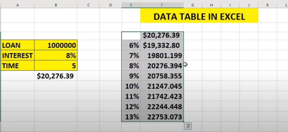
To use data table in Excel we have taken to find loan amount in Excel in the example below 

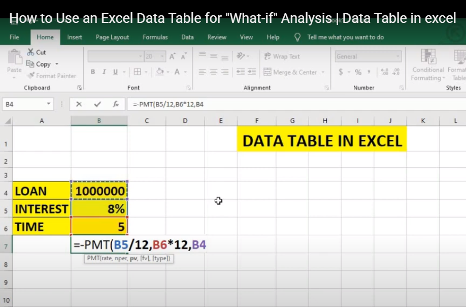
  • Loan Amount : 10,00000
  • Interest 8% yearly
  • Time : 5 years

First we use PMT function as shown below in the picture 

=PMT(rate, nper, pv, [fv], [type])


=PMT(rate/12, nper*12, pv, [fv], [type])

Note: here we divide rate by 12 and nper we divide 12 so we can get monthly installment of money . Fv blank type 0 or leave blank.

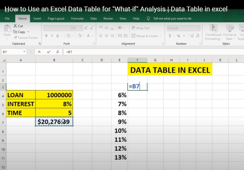
After finding the PMT.

Next is to create a table of rate like 6% 7% 8% etc.

  • Select PMT installment such as =B7.
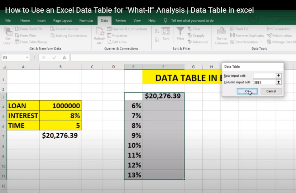
  • Select the table area.
  • Go to date table from table
  • Now in column select B7
  • Installment will appear.


what if analysis data table
excel data table analysis

SUMIFS

=SUMIFS is one of the “must-know” formulas for a data analyst. The common formula used is =SUM, but what if you need to sum values based on multiple criteria? SUMIFS is it. In the example below, SUMIFS is used to determine how much each product is contributing to top-line revenue.

Formula:

=SUMIF(RANGE,CRITERIA,[sum_range])


note: [sum_range] is optional

Use the formula

=SUMIF($A$4:$A$17,D3,$C$4:$C$17)

Use F4 Key for dollar sign.

and drag the formula till E8

SUMIFS Function in Excel

SUMIF function allows us to sum the data given based on associated criteria within the same data. However, the SUMIFs Function in Excel allows applying multiple criteria.

Formula used for the SUMIFS Function in Excel
“SUMIFS ( sum_range, criteria_range1, criteria1, [criteria_range2, criteria2, criteria_range3, criteria3, … criteria_range_n, criteria_n] )”


Type the formula and give it to SUMIFS($C$3:$C$16,$A$3:$A$16,D3,$B$3:$B$16,E3)

not drag the formula

10 common NumPy functions that are useful for data analysis: 10 common use cases for SQL in data analytics 10 commonly used Matplotlib commands for data analytics 10 different between SQL and No SQL 10 steps that show how data analytics is changing the banking industry: 10 steps to learn SQL for Data Analytics 10 steps to start career in data science 10 ways data analytics can be used in addressing climate change: 10 ways data analytics is changing healthcare 10 ways in which data analytics could change the pharmaceutical industry