

Table of Contents
ToggleBy Vista Academy • Updated • 6 min read
Data Visualization Basics
Matplotlib एक Python की सबसे लोकप्रिय डेटा विज़ुअलाइज़ेशन लाइब्रेरी है, जिसका उपयोग ग्राफ, चार्ट और इमेज को प्लॉट करने के लिए किया जाता है। चाहे आप beginner हों या data science सीख रहे हों, matplotlib python library आपको powerful visual reports बनाने में मदद करती है। यह सेक्शन Matplotlib, Pyplot, Numpy और Pandas के साथ visualization concepts को clear करता है।
pyplot की मदद से line, bar, pie charts बनाना
अब आगे आप सीखेंगे कि Matplotlib को कैसे install करें,
import matplotlib.pyplot as plt का सही उपयोग कैसे करें,
और इसे Pandas DataFrame के साथ कैसे use किया जाता है।
चलिए visualizations की इस exciting journey की शुरुआत करते हैं!

plt.plot(x, y) in MatplotlibBasic Plotting with Pyplot
The matplotlib.pyplot.plot(x, y) function is used to generate a simple
line plot from two arrays — x and y.
x represents values on the x-axis, while y represents values on the y-axis.
Both arrays must be of equal length but can contain any number of elements.
Here’s a practical example of how to create a line graph in Python using Matplotlib and NumPy:
import matplotlib.pyplot as plt
import numpy as np

# Generate sample data
x = np.linspace(0, 10, 100)
y = np.sin(x)

# Create the line plot
plt.plot(x, y)

# Add labels and title
plt.xlabel('x')
plt.ylabel('y')
plt.title('Sin Wave')

# Display the plot
plt.show()
In this example:
x contains 100 evenly spaced values between 0 and 10 using np.linspace().y stores the sine values of these x-points using np.sin().plt.plot(x, y) draws the line graph.xlabel, ylabel, and title.plt.show() displays the final plot on screen.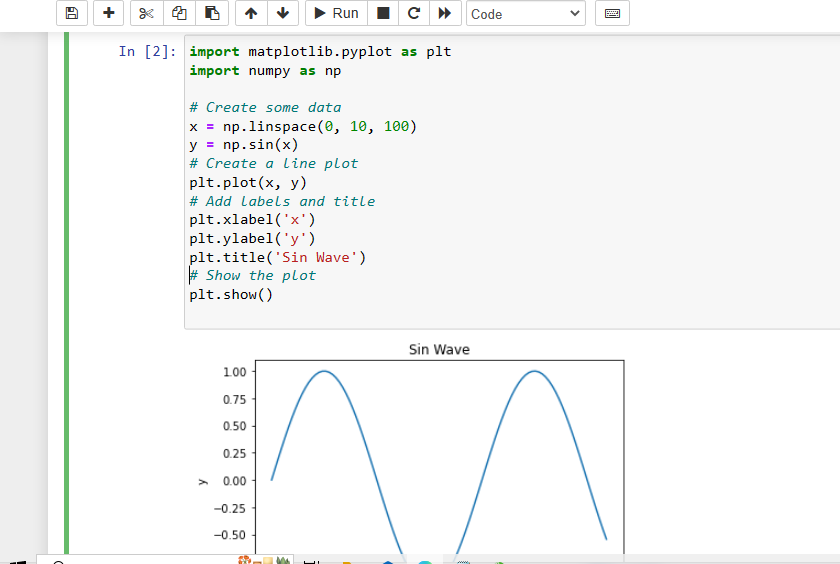
plt.xlabel()Axis Labeling in Pyplot
To label the x-axis of a plot in Python, use the
Matplotlib command plt.xlabel("your-label").
The text inside the function appears directly below the x-axis of your chart.
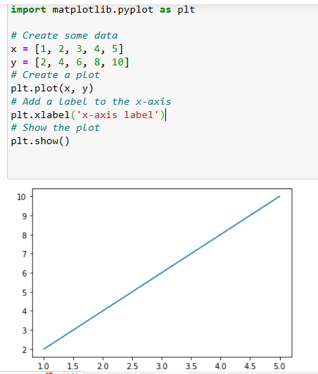
Below is an example demonstrating how to add an x-axis label using
plt.xlabel():
import matplotlib.pyplot as plt

# Sample data
x = [1, 2, 3, 4, 5]
y = [2, 4, 6, 8, 10]

# Create the plot
plt.plot(x, y)

# Add x-axis label
plt.xlabel("x-axis label")

# Show the plot
plt.show()
In this example:
plt.plot(x, y) generates the line graph.plt.xlabel("x-axis label") places a label below the x-axis.plt.show() displays the final chart with the label.You can customize the x-axis label using additional parameters such as font size, color, and style. This helps make your charts more readable and presentation-friendly, especially in analytics reports.
plt.ylabel()Axis Labeling in Python Charts
To add a label to the y-axis in a Matplotlib chart, use
plt.ylabel("label-text").
The text you provide inside this function appears along the vertical axis of your chart.
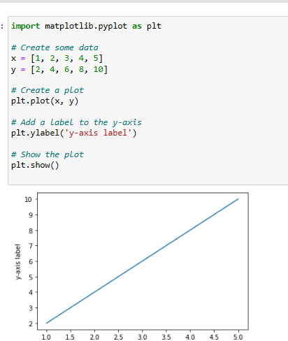
Here’s an example demonstrating how to label the y-axis using Matplotlib:
import matplotlib.pyplot as plt

# Sample data
x = [1, 2, 3, 4, 5]
y = [2, 4, 6, 8, 10]

# Create the plot
plt.plot(x, y)

# Add y-axis label
plt.ylabel("y-axis label")

# Show the plot
plt.show()
In this example:
plt.plot(x, y) creates the line graph.plt.ylabel("y-axis label") adds a vertical y-axis label.plt.show() displays the graph window with the labeled axis.Adding axis labels is essential for clear and professional data visualizations. It helps viewers understand what each axis represents—especially useful in dashboards and analytics reports.
plt.title()Adding Titles to Charts
You can add a title to your plot in Python by using the Matplotlib command
plt.title("Your Title").
This text appears at the top of your chart and helps viewers quickly understand the purpose of the plotted data.
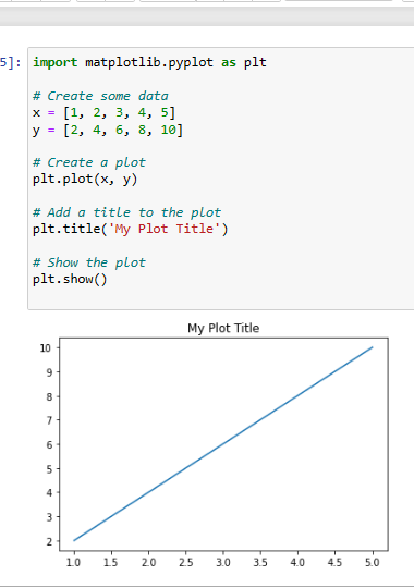
Here’s an example demonstrating how to use plt.title() with sample data:
import matplotlib.pyplot as plt

# Sample data
x = [1, 2, 3, 4, 5]
y = [2, 4, 6, 8, 10]

# Create the plot
plt.plot(x, y)

# Add a title
plt.title("My Plot Title")

# Show the plot
plt.show()
In this example:
plt.plot(x, y) generates a simple line chart from the lists.plt.title("My Plot Title") places a title above the graph.plt.show() displays the final chart with the title visible.
You can customize this title further using parameters like
fontsize, color, loc, and fontweight.
This helps make your plots presentation-ready and more suitable for analytics reports.
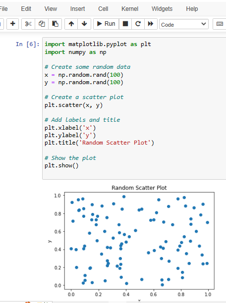
plt.scatter()Scatter Plot Visualization in Matplotlib
The Matplotlib function plt.scatter(x, y) is used to create a scatter plot,
a chart that displays individual data points.
Scatter plots are ideal for understanding relationships, trends, and data distribution.
The x array represents horizontal values, while the y array holds the vertical values.
Both arrays must have the same length.
Here’s an example showing how to create a basic scatter plot using NumPy and Matplotlib:
import matplotlib.pyplot as plt
import numpy as np

# Generate 100 random data points
x = np.random.rand(100)
y = np.random.rand(100)

# Create scatter plot
plt.scatter(x, y)

# Add axis labels and title
plt.xlabel('x-axis')
plt.ylabel('y-axis')
plt.title('Random Scatter Plot')

# Display the plot
plt.show()
In this example:
np.random.rand(100) generates 100 random values between 0 and 1.plt.scatter(x, y) plots these points on the scatter chart.plt.xlabel(), plt.ylabel(), plt.title() add context to the plot.plt.show() displays the final scatter plot window.Scatter plots are commonly used in data science and machine learning to identify patterns, clusters, correlations, and outliers. You can further customize marker size, shape, and color to make your visualizations more meaningful.
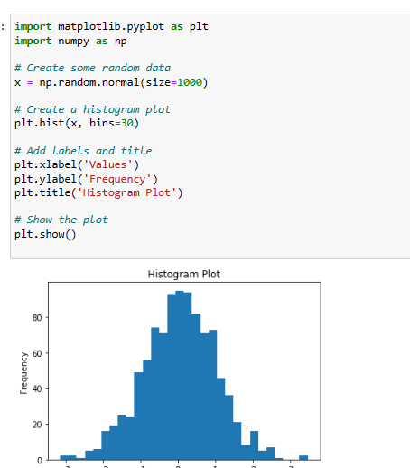
plt.hist()Frequency Distribution Visualization
A histogram is a chart used to represent the frequency distribution of a dataset.
In Matplotlib, you can create a histogram using
plt.hist(x, bins) where:
• x = dataset
• bins = number of bars or intervals
This helps group data into ranges and visualize how values are distributed.
Here’s a practical example of generating a histogram using Python and NumPy:
import matplotlib.pyplot as plt
import numpy as np

# Create random data from a normal distribution
x = np.random.normal(size=1000)

# Create histogram with 30 bins
plt.hist(x, bins=30, color='skyblue', edgecolor='black')

# Add labels and title
plt.xlabel('Values')
plt.ylabel('Frequency')
plt.title('Histogram Plot')

# Display the plot
plt.show()
In this example:
np.random.normal(size=1000) generates 1000 random values from a normal distribution.plt.hist(x, bins=30) divides data into 30 bins and plots the histogram.plt.xlabel(), plt.ylabel(), plt.title() add labels and a title.plt.show() displays the final plotted histogram.Histograms are extremely useful in data science, statistics, and machine learning for analyzing data distribution, skewness, variance, and patterns. You can customize colors, edge styling, transparency, and even add density curves.
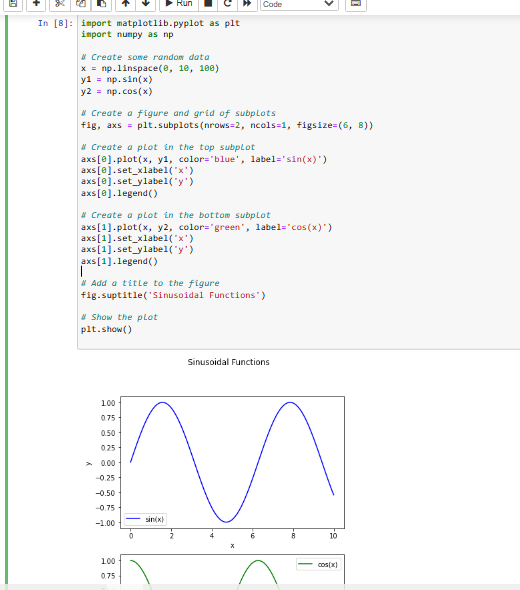
plt.subplots()Creating Grids of Charts in Matplotlib
The plt.subplots(nrows, ncols) function in Matplotlib is used to create
a grid of plots (called subplots).
You can define how many rows and columns of plots you want.
This technique is useful when you want to display multiple charts in a single figure for comparison.
Below is a step-by-step example showing how to create a vertical stack of two subplots:
import matplotlib.pyplot as plt
import numpy as np

# Create data
x = np.linspace(0, 10, 100)
y1 = np.sin(x)
y2 = np.cos(x)

# Create a 2-row, 1-column grid of subplots
fig, axs = plt.subplots(nrows=2, ncols=1, figsize=(6, 8))

# Plot sine curve on the first subplot
axs[0].plot(x, y1, color='blue', label='sin(x)')
axs[0].set_xlabel('x')
axs[0].set_ylabel('y')
axs[0].legend()

# Plot cosine curve on the second subplot
axs[1].plot(x, y2, color='green', label='cos(x)')
axs[1].set_xlabel('x')
axs[1].set_ylabel('y')
axs[1].legend()

# Add a common title
fig.suptitle('Sinusoidal Functions')

# Display the full plot
plt.show()
In this example:
plt.subplots(2, 1) creates two vertically stacked plots.axs[0] and axs[1] allow accessing and customizing each subplot individually.fig.suptitle() adds a common title across both subplots.figsize=(6, 8) sets the overall figure size (width × height in inches).
This method is extremely helpful when comparing multiple datasets side-by-side or top-to-bottom.
You can also create grids such as plt.subplots(2, 2) for a 2×2 layout, offering even more flexibility.
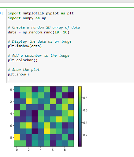
plt.imshow() in MatplotlibVisualizing 2D Data with Colormaps
The plt.imshow(data) function in Matplotlib is used to display a 2D array as an image.
It is commonly used to visualize heatmaps, grayscale images, matrices, filters, and more in data science and machine learning.
Here’s a simple example showing how to use plt.imshow() with randomly generated data:
import matplotlib.pyplot as plt
import numpy as np

# Create a 10x10 array of random values
data = np.random.rand(10, 10)

# Display the 2D array as an image
plt.imshow(data, cmap='viridis')  # Try cmap='hot', 'cool', 'gray', etc.

# Add colorbar for scale reference
plt.colorbar()

# Show the plot
plt.show()
🔍 Explanation:
np.random.rand(10, 10) creates a 10×10 matrix with random values between 0 and 1.plt.imshow(data) visualizes the matrix as an image.cmap defines the color palette (e.g., 'hot', 'viridis', 'gray').plt.colorbar() adds a scale bar to interpret image intensity values.This technique is widely used in image processing, machine learning, neural networks, and statistical analysis—for example, in confusion matrices, heatmaps, and convolutional filters.
plt.legend()Labels & Legends in Matplotlib
The plt.legend() command in Matplotlib is used to add a legend box to your chart.
A legend helps viewers understand what each plotted line, marker, or symbol represents by mapping them to
the labels assigned in your plot.
Below is an example demonstrating how to add a legend for sine and cosine curves:
import matplotlib.pyplot as plt
import numpy as np

# Generate x values
x = np.linspace(0, 10, 100)

# Generate y values
y1 = np.sin(x)
y2 = np.cos(x)

# Plot both lines with labels
plt.plot(x, y1, color='blue', label='sin(x)')
plt.plot(x, y2, color='green', label='cos(x)')

# Add legend to the plot
plt.legend()

# Add axis labels and title
plt.xlabel('x')
plt.ylabel('y')
plt.title('Trigonometric Functions')

# Display the plot
plt.show()
🔍 Explanation:
label='sin(x)' and label='cos(x)' give names to each plotted line.plt.legend() automatically creates a legend box using these labels.plt.legend(loc='upper right'), 'lower left', 'center', etc.
Legends are essential when visualizing multiple datasets in a single figure. They improve clarity and readability, especially when color-coded lines or markers represent different variables, functions, or models.

Why Matplotlib is essential for plotting in Python
Line charts, histograms, bar plots, scatter, polar and even 3D—Matplotlib covers every analytical need.
Control colors, fonts, labels, grid-lines and legends to create presentation-ready visuals.
Well-established library with active contributors, docs, and tons of tutorials.
Directly visualize NumPy arrays and Pandas DataFrames without extra conversion.
Works on Windows, macOS, and Linux — portable code for every environment.
Zoom, pan and interact using Matplotlib’s backends (TkAgg, Qt5Agg) or interactive tools.
Integrate plots into PyQt, Tkinter or wxPython GUIs to build data-driven apps.
Export to PNG, JPG, SVG or PDF in high resolution for reports and presentations.
Continuous updates and improvements keep Matplotlib modern and reliable.
Official docs, tutorials, courses and community forums make it easy to learn Matplotlib.
Common questions beginners ask
pip install matplotlib
in your terminal or command prompt.
Vista Academy का Master Program in Data Science advanced topics में इन-डेप्थ ट्रेनिंग देता है — जैसे मशीन लर्निंग, AI, बिग-डेटा एनालिटिक्स और predictive modeling. Hands-on projects के साथ Python, R, SQL और TensorFlow सीखकर अपने career को मजबूत बनाइए।