Excel data analyst questions for interview in Data Analysis

How do you freeze panes in Excel?

Table of Contents

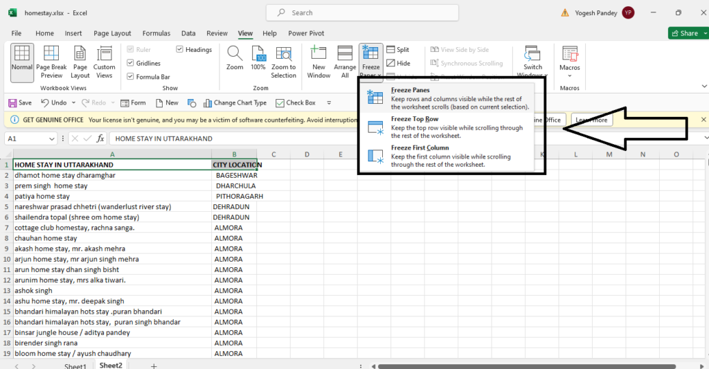
To freeze panes in Excel, follow these steps:

Select the cell below and to the right of the rows and columns you want to freeze. For example, if you want to freeze the top row and the first column, select the cell B2.
Go to the “View” tab on the Excel ribbon.
Click on the “Freeze Panes” dropdown menu.
Choose one of the options:
- “Freeze Panes” to freeze the selected rows and columns.
- “Freeze Top Row” to freeze the top row.
- “Freeze First Column” to freeze the first column.

For example, if you want to freeze the top row and the first column, select cell B2, then go to the “View” tab, click on “Freeze Panes”, and choose “Freeze Panes”. This action will freeze the top row and the first column, so when you scroll down or to the right, those frozen rows and columns will remain visible.

Explain the difference between absolute and relative cell references in Excel.

In Excel, cell references can be either absolute or relative, and understanding the difference between them is crucial for creating dynamic formulas that can be copied and pasted across different cells. Here’s an explanation along with examples:
Relative Cell Reference:
A relative cell reference changes based on the location of the formula when it’s copied to another cell.
When a formula with relative references is copied to another cell, the references adjust based on their new location relative to the original cell.
Relative references are indicated by the absence of any dollar signs ($) before the column letter and row number.
Example: Let’s say you have a formula in cell B2 that adds the values of cells A1 and A2: =A1 + A2. If you copy this formula to cell C3, it will adjust to =B2 + B3. This is because the formula maintains the same relative position to the new cell.
Absolute Cell Reference:
An absolute cell reference remains constant, regardless of where the formula is copied.
When a formula with absolute references is copied to another cell, the references remain fixed.
Absolute references are indicated by dollar signs ($) before the column letter and row number, like $A$1.
Example: Let’s say you have a formula in cell B2 that multiplies the value in cell A1 by 10: =$A$1 * 10. If you copy this formula to cell C3, it will still refer to cell A1, not C3 or any other cell.
Mixed Cell Reference:
Mixed references contain a combination of relative and absolute references, either the column or the row is fixed.
Example: $A1 is an absolute column reference (column A remains constant), but the row reference is relative (will change when copied to a different row). Similarly, A$1 is an absolute row reference (row 1 remains constant), but the column reference is relative (will change when copied to a different column).
Understanding these reference types allows you to create flexible and dynamic formulas in Excel.

How can you remove duplicates from a dataset in Excel?

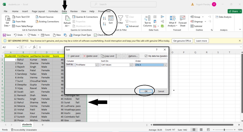
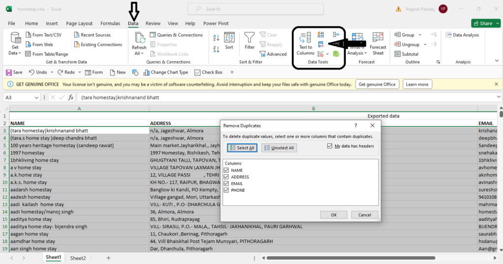
To remove duplicates from a dataset in Excel, you can use the built-in “Remove Duplicates” feature. Here’s how:

Select the Data:
Highlight the range of cells or columns that contain the dataset from which you want to remove duplicates.
Access the Remove Duplicates Dialog Box:
Go to the “Data” tab on the Excel ribbon.
Click on “Remove Duplicates”:
In the “Data Tools” group, you’ll find the “Remove Duplicates” button. Click on it.
Choose Columns:
A dialog box will appear showing all the columns in your selected range. Excel will automatically check all columns.
Uncheck any columns where you don’t want to remove duplicates based on the entire row’s content.
Confirm and Remove:
Click “OK” to remove duplicates based on the selected columns.
Excel will remove duplicate rows and keep only the unique records.
After these steps, Excel will remove duplicate rows from your dataset based on the criteria you selected. Remember that this action is permanent and cannot be undone, so it’s always a good idea to make a backup of your data before removing duplicates, especially if you’re working with a large dataset or if the data is critical.

What is the VLOOKUP function used for, and how does it work?

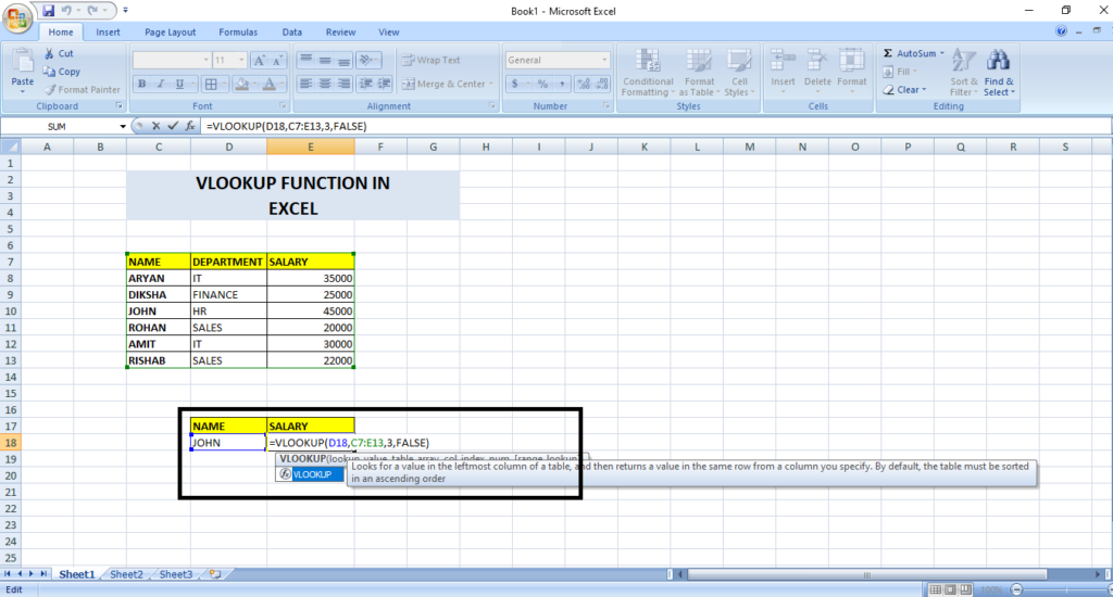
The VLOOKUP function in Excel is used to search for a value in the first column of a range (table) and return a value in the same row from a specified column. It stands for “Vertical Lookup.”
Here’s how it works:
Syntax:
The basic syntax of the VLOOKUP function is:

 =VLOOKUP(lookup_value, table_array, col_index_num, [range_lookup]).

Parameters:
lookup_value: The value you want to search for.
table_array: The range of cells that contains the data. The first column of this range is searched for the lookup_value.
col_index_num: The column number in the table_array from which to retrieve the matching value.
range_lookup: Optional parameter. If set to TRUE or omitted, it assumes the closest match. If set to FALSE, it looks for an exact match.

Example:
Suppose you have a table with employee names in column A and their corresponding salaries in column B. If you want to find the salary of an employee named “John,” you could use the formula:
=VLOOKUP(“John”, A1:B10, 2, FALSE)
This formula will search for “John” in the first column of the range A1:B10 and return the value from the second column (salary).
Overall, the VLOOKUP function is handy for looking up and retrieving information from large datasets, such as databases or tables, based on a specific criterion.

Describe the difference between CONCATENATE and CONCAT functions in Excel.

The main difference between the CONCATENATE and CONCAT functions in Excel lies in their usability and compatibility with newer versions of Excel.
CONCATENATE Function:
CONCATENATE has been available in Excel for a long time.
It allows you to concatenate (join together) multiple strings or values into one single string.
You need to list each item individually as arguments within the function.
Example: =CONCATENATE(“Hello “, “world”) returns “Hello world”.
CONCAT Function:
CONCAT was introduced in Excel 2016 and later versions.
It also concatenates multiple strings or values into one single string.
CONCAT can handle ranges and arrays directly, making it more versatile and efficient.
Example: =CONCAT(“Hello “, “world”) also returns “Hello world”.

In summary, CONCATENATE is the traditional method of concatenating strings, while CONCAT offers a more concise and versatile approach, especially for handling larger datasets or arrays of values.

How do you create a pivot table in Excel?

To create a pivot table in Excel, follow these steps:
1. Prepare Your Data:
Ensure your data is organized in a tabular format with columns and rows.
Include headers for each column.
2. Select Your Data:
Click anywhere within your dataset.
3. Insert PivotTable:
Go to the “Insert” tab on the Excel ribbon.
4. Click on PivotTable:
Click on the “PivotTable” button.
This will open the “Create PivotTable” dialog box.
5. Choose Your Data Range:
Ensure the correct range is selected in the “Select a table or range” field.
You can also manually enter the range if it’s not automatically detected.
6. Choose Location for Your PivotTable:
Choose where you want to place your PivotTable: either a new worksheet or an existing one.
Select “New Worksheet” to place the PivotTable on a new sheet.
7. Click OK:
Click the “OK” button in the “Create PivotTable” dialog box.
Excel will create a blank PivotTable on the selected location.
8. Customize Your PivotTable:
Drag fields from the “PivotTable Field List” to the areas below:
Rows: Fields placed here become the rows in your PivotTable.
Columns: Fields placed here become the columns in your PivotTable.
Values: Fields placed here are summarized with calculations like sum, count, average, etc.
Filters: Fields placed here can filter data in your PivotTable.
You can rearrange, remove, or add fields as needed to customize your PivotTable.
Refresh Data (If Needed):
If your source data changes, you may need to refresh your PivotTable to reflect those changes.
Right-click on the PivotTable and select “Refresh” to update it with the latest data.
By following these steps, you can create a PivotTable in Excel to analyze and summarize your data efficiently.

What is conditional formatting, and how can it be applied in Excel?

Conditional formatting in Excel is a feature that allows you to format cells based on specific conditions or criteria. This makes it easier to visually identify trends, patterns, or outliers in your data. Here’s how you can apply conditional formatting in Excel:
1. Select Your Data:
Highlight the range of cells or columns where you want to apply conditional formatting.
2. Access Conditional Formatting Options:
Go to the “Home” tab on the Excel ribbon.
Click on the “Conditional Formatting” dropdown menu.
3. Choose a Formatting Rule:
Select one of the predefined formatting rules from the menu, such as “Highlight Cells Rules” or “Top/Bottom Rules.”
Alternatively, you can create a custom rule by selecting “New Rule” from the dropdown menu.
4. Set the Condition:
In the dialog box that appears, specify the condition or criteria for the formatting rule.
For example, you can choose to format cells that are greater than a certain value, contain specific text, are within a certain date range, etc.
5. Choose Formatting Options:
After setting the condition, choose the formatting options you want to apply to cells that meet the condition.
This could include changing the font color, fill color, font style, borders, etc.
6. Preview and Apply:
Preview how your data will look with the selected formatting options.
Once satisfied, click “OK” to apply the conditional formatting to your selected range of cells.
7. Manage Rules (Optional):
You can manage existing conditional formatting rules by going to the “Conditional Formatting” dropdown menu and selecting “Manage Rules.”
Here, you can edit, delete, or reorder existing rules as needed.
8. Review and Adjust:
Review your formatted data and make adjustments as necessary.
You can always go back and modify the formatting rules or add new ones as your data analysis needs evolve.
By applying conditional formatting in Excel, you can visually highlight important information, trends, or outliers in your data, making it easier to interpret and analyze.

Explain the purpose of the IF function in Excel and provide an example.

The IF function in Excel allows you to perform logical tests and return different values based on whether the test evaluates to true or false. Its primary purpose is to make decisions within a formula. Here’s how it works:
Syntax:
=IF(logical_test, value_if_true, value_if_false)
logical_test: This is the condition you want to test. It could be a comparison, such as “A1>B1”, or any expression that can be evaluated as true or false.
value_if_true: This is the value that Excel returns if the logical_test evaluates to true.
value_if_false: This is the value that Excel returns if the logical_test evaluates to false.
Example: Suppose you have a column of exam scores in cells A1:A10, and you want to assign a grade of “Pass” if the score is greater than or equal to 70, and “Fail” otherwise. You can use the IF function to achieve this:
=IF(A1>=70, “Pass”, “Fail”)
If the score in cell A1 is 80, the formula will return “Pass”.
If the score in cell A1 is 60, the formula will return “Fail”.
This allows you to dynamically assign values or perform different calculations based on specific conditions in your Excel spreadsheet.

How do you transpose data in Excel?

To transpose data in Excel means to switch the orientation of rows and columns. Essentially, you’re converting data from a horizontal layout to a vertical one, or vice versa. Here’s how you can transpose data:
Select the Data: Highlight the range of cells that you want to transpose.
Copy the Data: Right-click on the selected range and choose “Copy”, or use the keyboard shortcut Ctrl + C.
Choose the Destination: Click on the cell where you want to paste the transposed data. Ensure that there are enough rows and columns to accommodate the transposed data.
Transpose Option:
Right-click on the destination cell.
Choose “Paste Special” from the context menu.
In the Paste Special dialog box, check the “Transpose” option.
Click “OK”.
Alternatively:
Go to the Home tab on the Excel ribbon.
Click on the small arrow under the “Paste” button.
Select “Transpose” from the dropdown menu.
Confirm Transposition: After selecting the “Transpose” option, Excel will paste the transposed data into the selected destination cell. The rows and columns will be switched accordingly.
Review and Adjust: Review the transposed data to ensure it appears as desired. You may need to adjust column widths or row heights to accommodate the transposed data properly.
By following these steps, you can easily transpose data in Excel, switching between horizontal and vertical orientations as needed.

What is the purpose of the INDEX-MATCH function combination in Excel?

The purpose of the INDEX-MATCH function combination in Excel is to perform a lookup that offers more flexibility and power than traditional lookup functions like VLOOKUP or HLOOKUP.
INDEX function: It returns the value of a cell in a specific row and column of a range or array. You specify the array and the row and column numbers to retrieve the value.
MATCH function: It returns the relative position of an item in an array that matches a specified value. You specify the lookup value and the array to search within.
When used together, INDEX and MATCH allow you to perform lookups in Excel based on one or more criteria, without the limitations of VLOOKUP (which requires the lookup value to be in the first column of the table). This combination is particularly useful for performing lookups in more complex datasets or when the lookup value isn’t in the first column.
Here’s how it works:
MATCH function is used to find the position of the lookup value within a column or row.
INDEX function is then used to return the value from a corresponding row or column in the data range.
Example:
Suppose you have a table with product names in column A, and their corresponding prices in column B. You want to find the price of a product named “Widget”. You can use INDEX and MATCH as follows:
=INDEX(B:B, MATCH(“Widget”, A:A, 0))
In this formula:
MATCH(“Widget”, A:A, 0) finds the position of “Widget” in column A.
INDEX(B:B, …) returns the value from column B at the position found by MATCH.
This combination offers more versatility and power compared to VLOOKUP, especially in situations where the lookup value isn’t in the first column or when dealing with large datasets.

How can you protect cells or sheets in Excel?

In Excel, you can protect cells or entire sheets to prevent users from making changes to specific parts of a workbook. Here’s how to protect cells or sheets:
Protecting Cells:
Select Cells: First, select the cells you want to protect.
Right-click on the selected cells and choose Format Cells from the context menu.
In the Format Cells dialog box, go to the Protection tab.
Check the box that says Locked to prevent changes to these cells.
Click OK.
Now, protect the worksheet. Go to the Review tab on the Excel ribbon.
Click on Protect Sheet.
In the Protect Sheet dialog box, you can set a password if you want. You can also choose specific options such as allowing users to select locked cells or format cells.
Click OK and enter the password if prompted.
Protecting Sheets:
Go to the Review tab on the Excel ribbon.
Click on Protect Sheet.
In the Protect Sheet dialog box, you can set a password if you want. You can also choose specific options such as allowing users to select locked cells or format cells.
Click OK and enter the password if prompted.
By following these steps, you can protect cells or entire sheets in Excel to prevent unwanted changes to your workbook.

Describe the purpose of the SUMIF and SUMIFS functions in Excel.

he purpose of the SUMIF and SUMIFS functions in Excel is to sum values based on specific criteria or conditions. They allow you to perform conditional summing of data in a range based on one or multiple criteria. Here’s how they work:
SUMIF Function:
Purpose: The SUMIF function adds up values in a range that meet a single specified condition.
=SUMIF(range, criteria, [sum_range])
Parameters:
range: The range of cells that you want to evaluate against the criteria.
criteria: The condition that determines which cells to sum. It can be a number, expression, cell reference, or text.
sum_range (optional): The range of cells to sum if they meet the criteria. If omitted, Excel will sum the values in the range.
Example; =SUMIF(A1:A10, “>50”)
This formula sums all the values in the range A1:A10 that are greater than 50.
SUMIFS Function:
Purpose: The SUMIFS function adds up values in a range that meet multiple specified conditions.
=SUMIFS(sum_range, criteria_range1, criteria1, [criteria_range2, criteria2], …)
Parameters:
sum_range: The range of cells to sum.
criteria_range1, criteria_range2, etc.: The ranges to evaluate against their corresponding criteria.
criteria1, criteria2, etc.: The conditions that determine which cells to sum.
Example: =SUMIFS(B1:B10, A1:A10, “>50”, C1:C10, “<>Red”)
This formula sums all the values in the range B1:B10 where the corresponding cells in column A are greater than 50 and the cells in column C are not equal to “Red”.
In summary, SUMIF is used when you have a single condition, while SUMIFS is used for multiple conditions. These functions are particularly useful for analyzing datasets and performing calculations based on specific criteria.

How do you create a chart or graph in Excel?

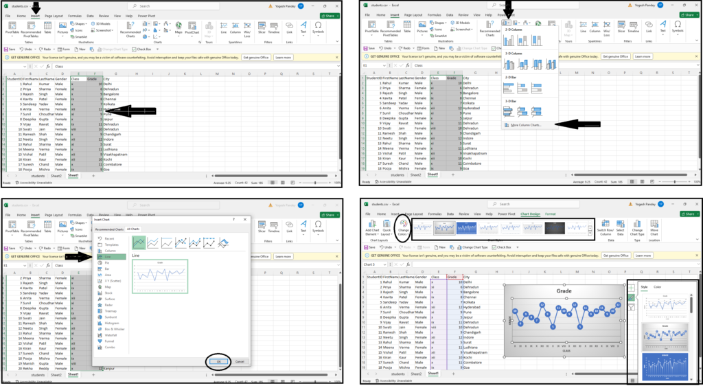
To create a chart or graph in Excel, follow these steps:
1. Select Data: Highlight the data you want to include in the chart. This could be a range of cells or a table.
2. Insert Chart: Go to the “Insert” tab on the Excel ribbon.
Choose Chart Type: Click on the type of chart you want to create from the “Charts” group. Common types include column, bar, line, pie, and scatter.
3. Customize Chart: Excel will insert a default chart based on your selected data. You can customize the chart by adding titles, axes labels, legends, and more. Right-click on any element of the chart to access formatting options.
4. Move and Resize: Click and drag the chart to move it to a different location on the worksheet. Resize by clicking and dragging the corners or edges of the chart.
5. Chart Tools: When you select the chart, the “Chart Tools” contextual tab will appear on the Excel ribbon. Use this tab to further customize the chart with design options, layout options, and chart styles.
6. Switch Data: If you want to change the data range used by the chart, click on the chart, and then click on the “Design” tab under “Chart Tools.” In the “Data” group, click on “Select Data” and update the data range as needed.
7. Refresh Data: If your source data changes, you may need to refresh the chart to reflect those changes. Right-click on the chart and select “Refresh” or click on the “Refresh Data” button in the “Data” group under “Chart Tools.”
By following these steps, you can create a chart or graph in Excel to visually represent your data and make it easier to understand and analyze.

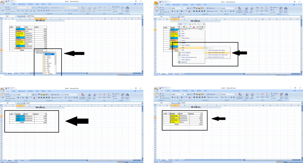
Explain how to use the SUBTOTAL function in Excel.

The SUBTOTAL function in Excel is used to perform calculations on a filtered range or dataset, excluding other subtotal results. It’s often used in conjunction with filtered lists or tables to calculate results dynamically.

=SUBTOTAL(function_num, ref1, [ref2], ...)

function_num: A number that specifies which function to use for the calculation (e.g., 1 for AVERAGE, 2 for COUNT, 9 for SUM, etc.).
ref1, ref2, …: References to the ranges or cells you want to include in the calculation.
Example: Suppose you have a list of numbers in cells A1:A10, and you’ve filtered out some of the rows. If you want to sum only the visible (filtered) numbers, you can use:

=SUBTOTAL(9, A1:A10)

Here, “9” represents the SUM function, and A1:A10 is the range of numbers. The SUBTOTAL function will calculate the sum of only the visible (filtered) numbers in the range.

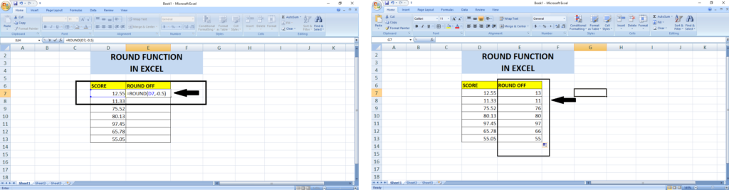
What is the purpose of the ROUND function in Excel?

The purpose of the ROUND function in Excel is to round a number to a specified number of digits. It allows you to control the precision or formatting of numerical values.

=ROUND(number, num_digits)

number: The number you want to round.
num_digits: The number of digits to which you want to round the number. If positive, it rounds to the right of the decimal point; if negative, it rounds to the left of the decimal point.
Example: Suppose you have a number 3.4567 in cell A1, and you want to round it to two decimal places. You can use:

=ROUND(A1, 2)

This formula will round the number to 3.46.

How do you create a drop-down list in Excel?

To create a drop-down list in Excel, you can use the Data Validation feature. Here’s how:
Select the Cell(s): Click on the cell or cells where you want the drop-down list to appear.
Go to Data Validation:
Go to the “Data” tab on the Excel ribbon.
Click on “Data Validation” in the “Data Tools” group.
Choose Data Validation:
In the Data Validation dialog box, go to the “Settings” tab.
Select “List”:
In the “Allow” dropdown menu, select “List”.
Enter the List Source:
In the “Source” field, enter the list of items you want to appear in the drop-down list. You can type the items directly or reference a range of cells that contain the items.
Optional: Enable Error Alert (Optional):
If you want to show an error message when users try to enter values not in the list, go to the “Error Alert” tab and customize the error message settings.
Click OK:
Click “OK” to apply the data validation settings.
Now, when you click on the cell(s) where you applied data validation, a drop-down arrow will appear. Clicking on this arrow will show the list of items you entered, and users can select from these options.
This method allows you to create a drop-down list in Excel, making data entry more efficient and reducing errors.

Describe how to use the TEXT function in Excel.

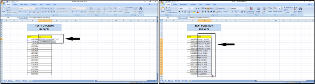
The TEXT function in Excel is used to convert a numeric value into text with a specified format. Here’s how to use it:

=TEXT(value, format_text)

value: The numeric value you want to convert to text.
format_text: The format you want to apply to the text.
Example: Suppose you have a date in cell A1 (e.g., 01/15/2024), and you want to display it as “January 15, 2024”. You can use:

=TEXT(A1, "mmmm dd, yyyy")

This formula will convert the date into text with the specified format.

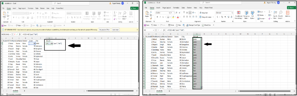
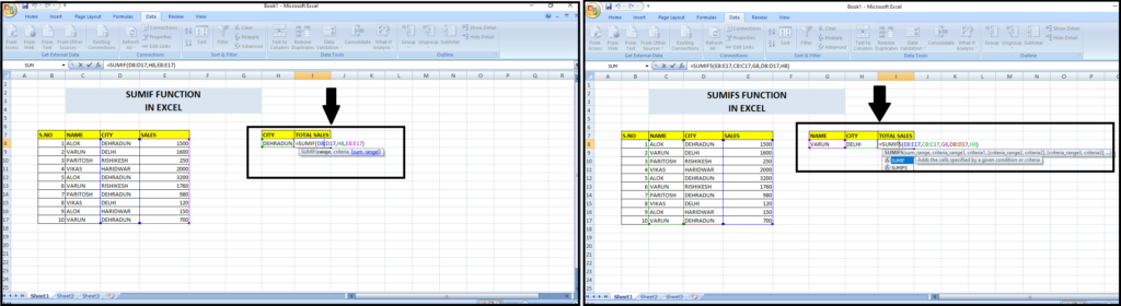
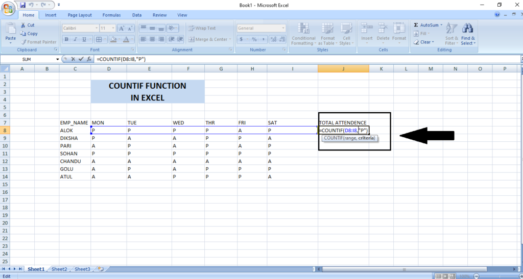
What is the purpose of the COUNTIF function in Excel?

The purpose of the COUNTIF function in Excel is to count the number of cells within a range that meet a specified condition or criteria.

=COUNTIF(range, criteria)

range: The range of cells you want to count.
criteria: The condition or criteria that determines which cells to count.
Example: Suppose you have a list of numbers in cells A1:A10, and you want to count how many of them are greater than 50. You can use:

=COUNTIF(A1:A10, ">50")

This formula will count the number of cells in the range A1:A10 that are greater than 50.

How do you find and replace data in Excel?

To find and replace data in Excel, follow these steps:
1. Select the Data Range:
Click on any cell within the range of data where you want to perform the find and replace operation.
2. Open the Find and Replace Dialog Box:
Press the keyboard shortcut Ctrl + H. Alternatively, you can go to the “Home” tab on the Excel ribbon, click on the “Find & Select” dropdown menu in the “Editing” group, and then select “Replace”.
3. Enter the Text to Find:
In the “Find what” field of the dialog box, type the text you want to find.
4. Enter the Replacement Text:
In the “Replace with” field, type the text you want to replace the found text with.
5. Choose Options (Optional):
You can choose additional options such as matching case, finding entire cells only, or searching within formulas by clicking the “Options >>” button.
6. Perform Find and Replace:
Click on the “Find Next” button to find the next occurrence of the search text.
Click on the “Replace” button to replace the found text with the replacement text. You can also click on “Replace All” to replace all occurrences in the selected range.
7. Review Changes:
Excel will notify you about each replacement it makes. You can review each change before proceeding.
8. Close Dialog Box:
Once you’ve finished finding and replacing, click on the “Close” button to close the Find and Replace dialog box.
By following these steps, you can find and replace data in Excel efficiently, whether it’s a single occurrence or multiple occurrences within a range of cells.

Explain the purpose of the NETWORKDAYS function in Excel.

The purpose of the NETWORKDAYS function in Excel is to calculate the number of working days (business days) between two dates, excluding weekends (Saturday and Sunday) and optionally, specified holidays.

=NETWORKDAYS(start_date, end_date, [holidays])

start_date: The start date of the period.
end_date: The end date of the period.
holidays: Optional. A range of dates representing holidays to exclude from the calculation.
Example: Suppose you want to calculate the number of working days between January 1, 2024, and January 15, 2024, excluding the holidays listed in cells A1:A5. You can use:

=NETWORKDAYS("2024-01-01", "2024-01-15", A1:A5)

This formula will return the number of working days between the specified dates, excluding weekends and the holidays listed in the range A1:A5.

How can you calculate the average, maximum, and minimum values in a dataset using Excel functions?

You can calculate the average, maximum, and minimum values in a dataset using the following Excel functions:
Average: Use the AVERAGE function.
Syntax: =AVERAGE(range)
Example: =AVERAGE(A1:A10) calculates the average of values in cells A1 through A10.
Maximum: Use the MAX function.
Syntax: =MAX(range)
Example: =MAX(A1:A10) returns the maximum value from cells A1 through A10.
Minimum: Use the MIN function.
Syntax: =MIN(range)
Example: =MIN(A1:A10) returns the minimum value from cells A1 through A10.
These functions provide a quick and easy way to analyze datasets and obtain summary statistics in Excel.

Describe how to use the Goal Seek feature in Excel.

The Goal Seek feature in Excel allows you to find the value of a specific cell that will achieve a desired result in another cell by changing the value of a third cell. Here’s how to use it:
Identify Your Goal:
Determine the desired result that you want to achieve in a specific cell.
Select Goal Seek:
Go to the “Data” tab on the Excel ribbon.
Click on What-If Analysis:
In the “Data Tools” group, click on “What-If Analysis”.
Choose Goal Seek:
Select “Goal Seek” from the dropdown menu.
Set Up Goal Seek Dialog Box:
In the Goal Seek dialog box, you’ll see three input fields:
“Set cell”: Enter the reference of the cell containing the formula you want to solve for.
“To value”: Enter the desired result or value you want to achieve in the set cell.
“By changing cell”: Enter the reference of the cell that you want to change to reach the desired result.
Run Goal Seek:
After entering the necessary information in the Goal Seek dialog box, click “OK”.
Excel will perform calculations to find the value of the “By changing cell” that will result in the desired value in the “Set cell”.
Review Results:
Excel will display the calculated value that achieves the desired result in the “Set cell” based on the value in the “By changing cell”.
Accept or Reject Solution:
You can choose to accept or reject the solution provided by Goal Seek. If you accept it, Excel will update the value in the “By changing cell” accordingly.
By following these steps, you can use the Goal Seek feature in Excel to find the value of a cell needed to achieve a specific result in another cell by adjusting the value of a third cell.

What is the purpose of the CONCATENATE function in Excel?

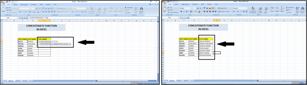
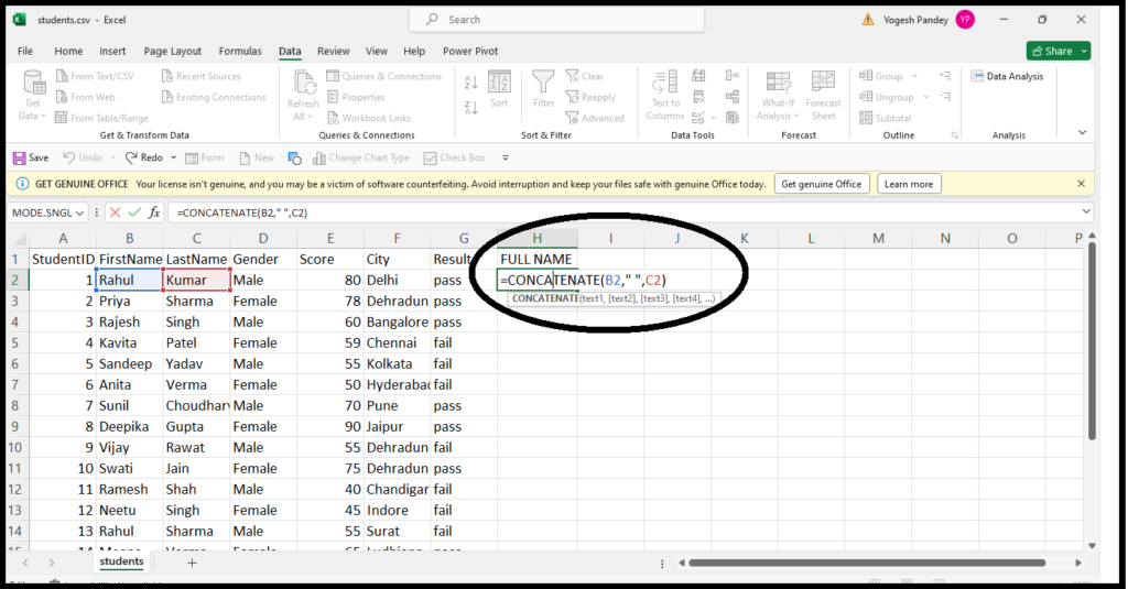
The CONCATENATE function in Excel is used to combine multiple strings or values into one single string. It is primarily used to concatenate, or join together, text from different cells or static text strings.

=CONCATENATE(text1, [text2], ...)

text1, text2, …: The text strings or cell references you want to concatenate.
Example: Suppose you have first name and last name in cells A1 and B1 respectively, and you want to concatenate them into one cell. You can use:

=CONCATENATE(A1, " ", B1)

This formula will combine the contents of cells A1 and B1, separated by a space, into one single string.

How do you use the Data Validation feature in Excel?

The Data Validation feature in Excel allows you to control what type of data users can enter into a cell or range of cells. Here’s how to use it:
Select the Cell(s):
Click on the cell or range of cells where you want to apply data validation.
Go to Data Validation:
Go to the “Data” tab on the Excel ribbon.
Click on Data Validation:
Click on the “Data Validation” button in the “Data Tools” group.
Set Validation Criteria:
In the Data Validation dialog box, go to the “Settings” tab.
Choose Validation Criteria:
Choose the type of data you want to allow in the cell(s) from the “Allow” dropdown menu. Options include whole numbers, decimals, dates, times, text length, and custom formulas.
Enter Criteria:
Based on the type of data selected, enter specific criteria. For example, if you choose “Whole number”, you can specify a minimum and maximum value.
Input Message (Optional):
Go to the “Input Message” tab to enter a message that will appear when the cell is selected. This can provide instructions or guidance on what type of data to enter.
Error Alert (Optional):
Go to the “Error Alert” tab to set up an error message that appears if the user enters data that does not meet the validation criteria.
Click OK:
Once you have set up the validation criteria, click “OK” to apply data validation to the selected cell(s).
Now, users will be restricted to entering only the type of data allowed by the validation criteria you set up. If they attempt to enter invalid data, an error message will appear according to the settings you specified.

Explain the purpose of the COUNTIFS function in Excel.

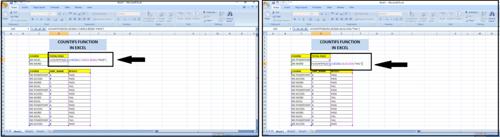
The purpose of the COUNTIFS function in Excel is to count the number of cells that meet multiple specified criteria across multiple ranges.

=COUNTIFS(criteria_range1, criteria1, [criteria_range2, criteria2], ...)

criteria_range1, criteria_range2, …: The ranges of cells to evaluate against their corresponding criteria.
criteria1, criteria2, …: The conditions or criteria that determine which cells to count.
Example: Suppose you have a dataset with sales data, and you want to count the number of sales where the product is “Apples” and the sales amount is greater than 100. You can use:

=COUNTIFS(A1:A10, "Apples", B1:B10, ">100")

This formula will count the number of cells in the range A1:A10 where the product is “Apples” and in the range B1:B10 where the sales amount is greater than 100.

How do you create a formula in Excel?

To create a formula in Excel, follow these general steps:

Select the Cell:
- Click on the cell where you want the result of your formula to appear.
Start with an Equal Sign:
- Begin your formula by typing an equal sign (=) into the selected cell. This signals to Excel that you’re entering a formula.
Enter the Formula:
- Enter the formula using cell references, operators, and functions as needed. You can use arithmetic operators like +, -, *, /, and ^ for addition, subtraction, multiplication, division, and exponentiation respectively. You can also use built-in functions like SUM, AVERAGE, IF, etc.
Press Enter:
- After entering your formula, press the Enter key on your keyboard. Excel will calculate the result of the formula and display it in the selected cell.

Example: If you want to add the values in cells A1 and B1, you would follow these steps:

Click on the cell where you want the result to appear (e.g., C1).
Type =A1+B1 into the cell.
Press Enter.
Excel will display the sum of the values in cells A1 and B1 in cell C1.

By following these steps, you can create and enter formulas in Excel to perform calculations and manipulate data according to your needs.

Describe the purpose of the LEFT, RIGHT, and MID functions in Excel.

The LEFT, RIGHT, and MID functions in Excel are used to extract substrings from a larger text string based on specific criteria, such as the number of characters or the starting position. Here’s a brief description of each function:
1. LEFT Function:
Purpose: Extracts a specified number of characters from the beginning (left side) of a text string.
=LEFT(text, num_chars)
Example: =LEFT(“Hello World”, 5)
This formula returns “Hello”, the first 5 characters from the left side of the text string “Hello World”.
2. RIGHT Function:
Purpose: Extracts a specified number of characters from the end (right side) of a text string.
=RIGHT(text, num_chars)
Example: =RIGHT(“Hello World”, 5)
This formula returns “World”, the last 5 characters from the right side of the text string “Hello World”.
3. MID Function:
Purpose: Extracts a specified number of characters from a text string, starting at a specified position.
=MID(text, start_num, num_chars)
Example; =MID(“Hello World”, 7, 5)
This formula returns “World”, starting from the 7th character and extracting the next 5 characters from the text string “Hello World”.
These functions are particularly useful for manipulating and extracting specific parts of text strings within Excel formulas.

How do you create a named range in Excel?

To create a named range in Excel, follow these steps:
Select the Range:
Highlight the range of cells that you want to name.
Go to the Formulas Tab:
Click on the “Formulas” tab on the Excel ribbon.
Click on Name Manager:
In the “Defined Names” group, click on “Name Manager”.
Click on New:
In the Name Manager dialog box, click on the “New” button.
Enter Name and Range:
In the “New Name” dialog box, enter a name for your range in the “Name” field.
In the “Refers to” field, Excel should automatically display the reference of the selected range you highlighted earlier. You can edit this reference if needed.
Click OK:
Click “OK” to create the named range.
Your named range is now created and can be used in formulas or data validation rules throughout your workbook. You can access and manage named ranges at any time by going to the “Formulas” tab, clicking on “Name Manager”, and selecting the desired named range.

What is the purpose of the HLOOKUP function in Excel?

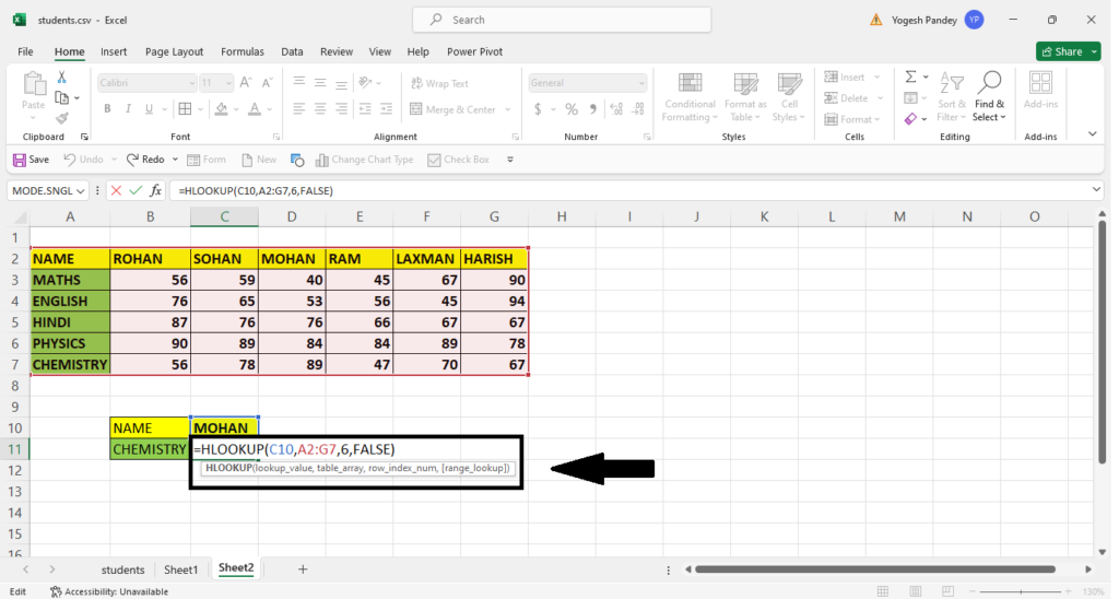
The purpose of the HLOOKUP function in Excel is to horizontally search for a value in the first row of a table or an array, and then return a value in the same column from a specified row number.

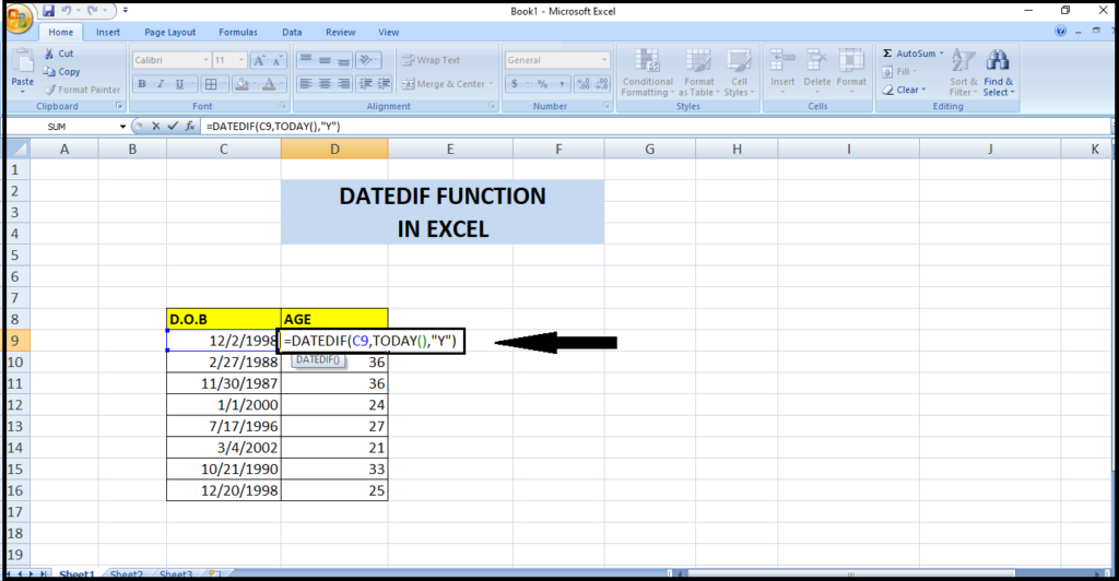
How do you create a formula to calculate the age based on the birthdate in Excel?

To calculate age based on the birthdate in Excel, you can use the following formula:

=DATEDIF(birthdate, TODAY(), "Y")

Replace “birthdate” with the cell reference containing the birthdate. This formula calculates the difference in years between the birthdate and the current date.

How would you calculate the standard deviation of a dataset in Excel?

To calculate the standard deviation of a dataset in Excel, you can use the STDEV function. Here’s how to do it:

Select a cell where you want the standard deviation to appear.
Type =STDEV( to start the function.
Select the range of data for which you want to calculate the standard deviation.
Close the parentheses ) and press Enter.

For example, if your data is in cells A1:A10, the formula would look like this: =STDEV(A1:A10). Excel will then calculate and display the standard deviation of the selected dataset.

What are array formulas in Excel? Provide an example.

Array formulas in Excel are formulas that perform multiple calculations on one or more items in an array. These formulas can return single or multiple results and are entered by pressing Ctrl + Shift + Enter instead of just Enter.

Here’s an example of an array formula:

Let’s say you have two columns of numbers in cells A1:A5 and B1:B5, and you want to calculate the sum of the products of corresponding numbers in each column.

You can use the following array formula to achieve this:

=SUM(A1:A5 * B1:B5)

After typing the formula, instead of pressing Enter, you press Ctrl + Shift + Enter. Excel will then calculate the sum of the products of the corresponding numbers in the two columns.

What are some common error types in Excel and how would you resolve them?

Common error types in Excel include:

#DIV/0!: Occurs when attempting to divide by zero.
#VALUE!: Occurs when using an incorrect data type in a formula or function.
#REF!: Occurs when referencing a cell that is not valid.
#NAME?: Occurs when Excel does not recognize text within a formula.
#NUM!: Occurs when a numeric value in a formula is invalid.
#N/A: Indicates that a value is not available.

To resolve these errors:

#DIV/0!: Check if the denominator is zero before performing division.
#VALUE!: Ensure that the data types used in formulas or functions are appropriate.
#REF!: Check and correct any invalid cell references.
#NAME?: Correct any misspelled function names or references.
#NUM!: Verify the numeric values used in the formula for validity.
#N/A: Check if the value is truly not available or if there’s a problem with the data source.

Additionally, using error-handling functions like IFERROR or IFNA can help manage errors by displaying custom messages or alternative values.

Can you explain the difference between "AND" and "OR" functions in Excel?

Certainly! The “AND” and “OR” functions in Excel are logical functions used to evaluate multiple conditions and return a TRUE or FALSE result based on the outcome of those conditions.

AND Function:
- The “AND” function returns TRUE if all of the specified conditions are TRUE.
- It returns FALSE if any of the specified conditions are FALSE.

Syntax: =AND(condition1, [condition2], ...)

Example: =AND(A1>10, B1<20, C1="Yes") returns TRUE only if cell A1 is greater than 10, cell B1 is less than 20, and cell C1 contains the text "Yes".

2. OR Function:

The “OR” function returns TRUE if at least one of the specified conditions is TRUE.
It returns FALSE if none of the specified conditions are TRUE.

Syntax: =OR(condition1, [condition2], ...)

Example: =OR(A1="Yes", B1="Yes", C1="Yes") returns TRUE if at least one of the cells A1, B1, or C1 contains the text "Yes".

In summary, “AND” evaluates all conditions and returns TRUE only if all conditions are met, while “OR” evaluates all conditions and returns TRUE if at least one condition is met.

How would you filter data in Excel?

To filter data in Excel, follow these steps:
Select the Data Range: Click on any cell within the data range you want to filter.
Open the Filter Menu: Go to the “Data” tab on the ribbon, then click on the “Filter” button. Alternatively, you can use the keyboard shortcut Ctrl + Shift + L.
Filter Options: Once the filter is applied, drop-down arrows will appear next to each column header. Click on the drop-down arrow of the column you want to filter.
Select Filter Criteria: In the drop-down menu, you can select specific items to filter by, sort options, or use search functionality to find specific values.
Apply Filter: Check or uncheck the boxes corresponding to the items you want to include or exclude from the filter. You can also use text filters, number filters, date filters, or custom filters based on your requirements.
Clear Filter: To clear the filter and display all data again, click on the drop-down arrow and select “Clear Filter” or click on the “Filter” button again to toggle off filtering.
By following these steps, you can easily filter data in Excel to view only the information that meets specific criteria.

What is conditional formatting and how is it useful in data analysis?

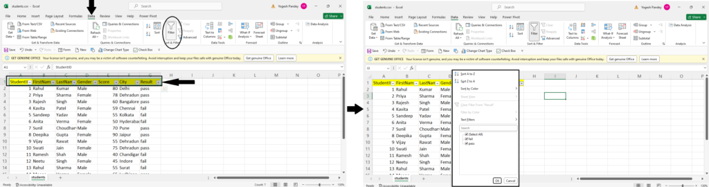
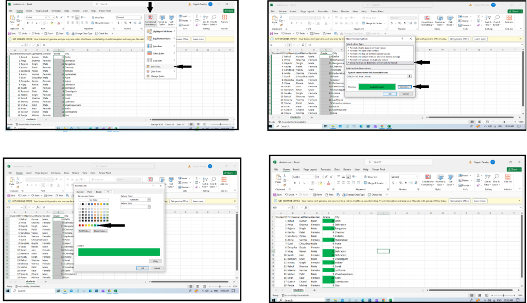
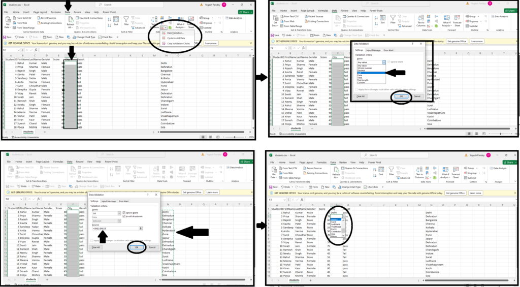
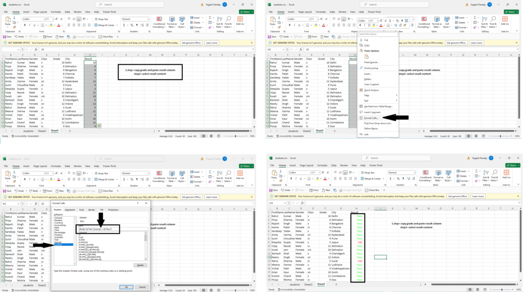
Conditional formatting is a feature in Excel that allows you to apply formatting (such as colors, icons, or data bars) to cells based on specified conditions. This feature helps to visually highlight important trends, patterns, or outliers within your data, making it easier to interpret and analyze.

Conditional formatting is useful in data analysis for several reasons:

Highlighting Key Data Points: You can use conditional formatting to highlight data points that meet certain criteria, such as values above or below a threshold, outliers, or specific text entries.
Identifying Trends and Patterns: By applying conditional formatting rules, you can quickly identify trends, patterns, or correlations in your data. For example, you can use color scales to visually represent the distribution of data values across a range.
Spotting Anomalies and Errors: Conditional formatting can help you identify anomalies or errors in your data, such as missing values, duplicates, or inconsistencies, by applying formatting that stands out from the rest of the data.
Improving Readability and Interpretation: By visually enhancing your data with conditional formatting, you can improve the readability and interpretation of your spreadsheets, making it easier for stakeholders to understand the insights and conclusions drawn from the data.
Conditional Formatting Based on Other Cells: You can also apply conditional formatting based on values in other cells, allowing you to create dynamic formatting that adjusts automatically as the underlying data changes.

Overall, conditional formatting is a powerful tool in data analysis that helps you visually explore and understand your data, identify important insights, and communicate findings effectively to others.

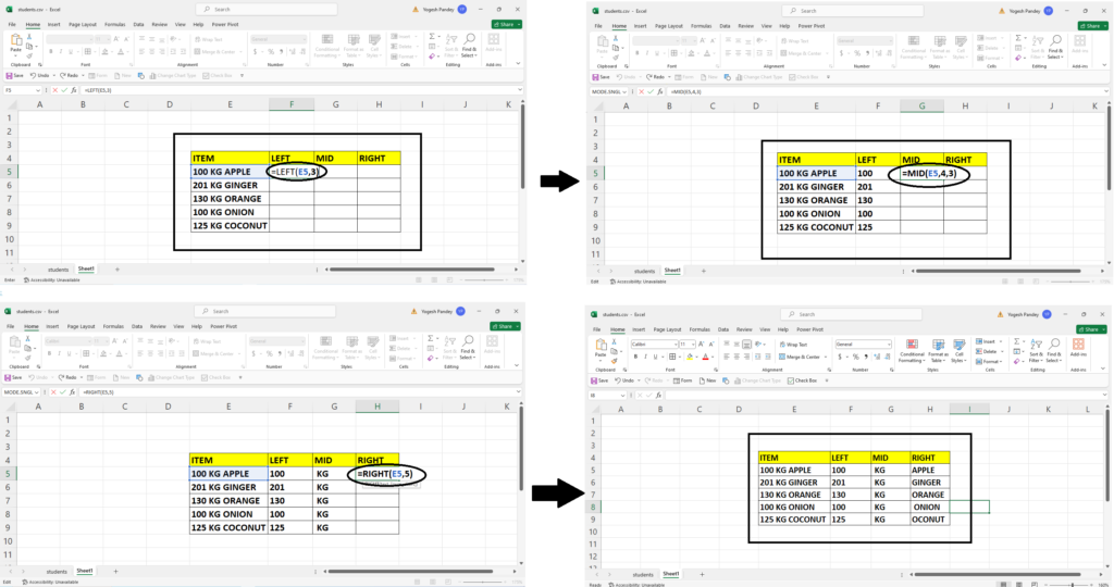
How do you use the FIND function in Excel?

The FIND function in Excel is used to locate the position of a specific character or substring within a text string. Here’s how you use it:

Syntax: FIND(find_text, within_text, [start_num])

find_text: The text you want to find within another text string.
within_text: The text string in which you want to search for find_text.
start_num (optional): The position in the within_text where you want to start searching. If omitted, the search starts at the beginning of the text.

Example: Suppose you have the text string “apple pie” in cell A1, and you want to find the position of the space character. You would use the FIND function like this:

=FIND(" ", A1)

This formula will return the position of the first space character in cell A1, which is 6 in this case.

You can also specify the start position from where you want to begin the search. For example:

=FIND("p", A1, 3)

This formula will find the position of the letter “p” in the text string starting from the third character, returning 6.

How would you calculate the compound interest in Excel?

To calculate compound interest in Excel, you can use the formula for compound interest, which is:

A=P×(1+r)n

Where:

$A$ is the future value of the investment/loan, including interest.
$P$ is the principal investment amount (the initial deposit or loan amount).
$r$ is the annual interest rate (in decimal).
$n$ is the number of periods the interest is compounded for.

In Excel, you can use the POWER function to raise (1 + r) to the power of $n$ and then multiply it by the principal $P$ to get the future value $A$ .

Here’s how you can do it step by step:

Determine the values of $P$ , $r$ , and $n$ .
Use the formula =P*(1+r)^n in a cell to calculate the future value $A$ , where $P$ , $r$ , and $n$ are replaced with your values.
Excel will automatically calculate the compound interest and display the result.

For example, let’s say you have $1000 as the principal amount, an annual interest rate of 5% (0.05 in decimal), and the interest is compounded annually for 3 years. The formula in Excel would be:

=1000*(1+0.05)^3

This will give you the future value of the investment after 3 years with compound interest.

What is the purpose of the RANK function in Excel?

The RANK function in Excel is used to determine the rank of a specified value in a list of values. It assigns a rank to a value based on its position relative to other values in the list.

Syntax: RANK(number, ref, [order])

number: The value for which you want to determine the rank.
ref: A reference to the list of values in which you want to rank the specified number.
order (optional): Specifies whether to rank the number in descending or ascending order. If omitted, the function ranks the number in descending order (largest value gets the highest rank).

The RANK function returns the rank of the specified number within the list of values.

For example, if you have a list of numbers in cells A1:A10 and you want to find the rank of the number in cell B1 within that list, you would use the formula:

=RANK(B1, $A$1:$A$10)

This formula would return the rank of the value in cell B1 relative to the values in cells A1:A10.

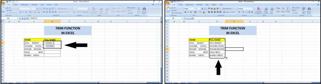
What is the purpose of the TRIM function in Excel?

The TRIM function in Excel is used to remove extra spaces from text, specifically leading and trailing spaces, as well as multiple consecutive spaces between words.

Its primary purpose is to clean up text data by removing unnecessary spaces that can sometimes be inadvertently included, which may cause issues when performing comparisons or analysis.

Syntax: TRIM(text)

text: The text string that you want to remove extra spaces from.

For example, if you have a text string with extra spaces like ” example text “, using the TRIM function will result in “example text”, with only single spaces between words and no leading or trailing spaces.

=TRIM(" example text ")

This function is particularly useful when dealing with imported data or user input, where extra spaces might be unintentionally included.

Explain the purpose of the PMT function in Excel.

The PMT function in Excel is used to calculate the periodic payment for a loan or investment based on constant payments and a constant interest rate. It helps in determining the amount of regular payments needed to pay off a loan or investment over a specified period.

Syntax: PMT(rate, nper, pv, [fv], [type])

rate: The interest rate per period.
nper: The total number of payment periods.
pv: The present value, or the initial principal amount of the loan or investment.
fv (optional): The future value, or the desired balance after the last payment is made. If omitted, it defaults to 0.
type (optional): The timing of payments: 0 for payments at the end of the period (default), or 1 for payments at the beginning of the period.

The PMT function returns a negative value, representing the outgoing payment.

For example, if you have a loan of $10,000 with an annual interest rate of 5%, to be paid off in 5 years, the formula to calculate the monthly payment would be:

=PMT(5%/12, 5*12, 10000)

This will give you the amount of the monthly payment required to pay off the loan over 5 years at an annual interest rate of 5%.

How do you create a custom number format in Excel?

To create a custom number format in Excel, follow these steps:
1. Select the Cell or Range: Click on the cell or range of cells that you want to apply the custom number format to.
2. Open the Format Cells Dialog Box:
Right-click on the selected cell(s) and choose “Format Cells…” from the context menu, OR
Go to the “Home” tab on the ribbon, click on the small arrow in the “Number” group to open the Format Cells dialog box.
3. Choose the Custom Category: In the Format Cells dialog box, select the “Number” tab if not already selected.
4. Create the Custom Format: In the Category list, select “Custom”. Then, in the “Type” field, enter your custom number format code.
Example custom number format codes:
To display numbers with thousand separators: #,##0
To display numbers with two decimal places: 0.00
To display negative numbers in red: #,##0.00;[Red](#,##0.00)
5. Apply the Custom Format: Click “OK” to apply the custom number format to the selected cell(s).
The custom number format will now be applied to the selected cell(s), displaying the numbers according to the format code you specified.

What is the purpose of the TRANSPOSE function in Excel?

The purpose of the TRANSPOSE function in Excel is to transpose or switch the orientation of a range of cells or an array. In other words, it converts rows into columns and columns into rows.

Syntax: TRANSPOSE(array)

array: The range of cells or array that you want to transpose.

The TRANSPOSE function is useful when you need to reorganize data from a horizontal layout to a vertical layout or vice versa. It can be particularly handy when working with large datasets or when you need to perform calculations or analysis on data that is structured differently from what is required.

For example, if you have data arranged in rows and you want to switch it to columns, or if you have data arranged in columns and you want to switch it to rows, you can use the TRANSPOSE function to quickly achieve this transformation.

How would you remove leading and trailing spaces from a cell in Excel?

To remove leading and trailing spaces from a cell in Excel, you can use the TRIM function. TRIM removes extra spaces from text except for single spaces between words. Here’s how:

Select the cell or range of cells from which you want to remove leading and trailing spaces.
Enter the formula =TRIM(cell) where “cell” is the reference to the cell containing the text with leading and trailing spaces.
Press Enter.

For example, if you have text with leading and trailing spaces in cell A1, you would enter =TRIM(A1) in another cell, and Excel will display the text without the extra spaces.

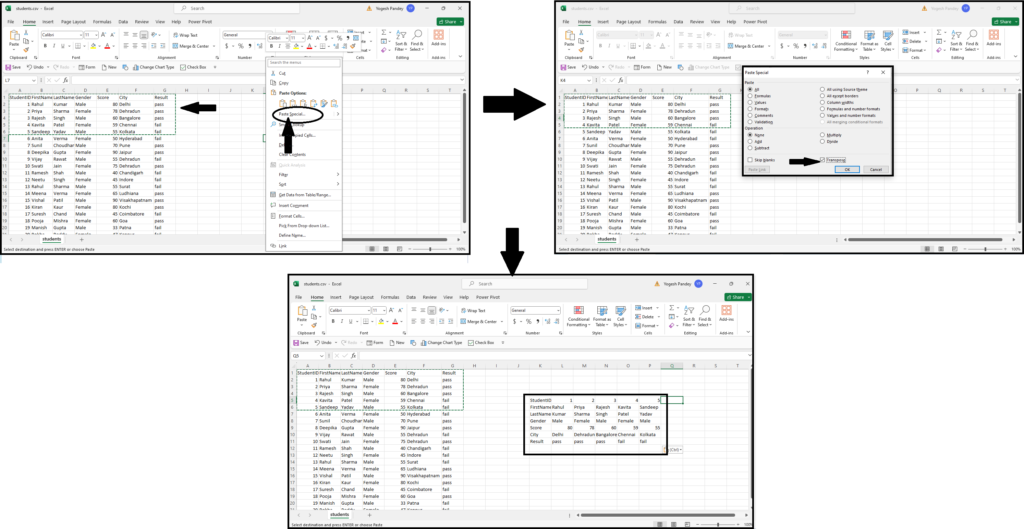
You can also directly replace the original text with the trimmed text by copying the trimmed text and using “Paste Special” > “Values” to paste it over the original text. This will replace the original text with the trimmed text, removing the leading and trailing spaces.

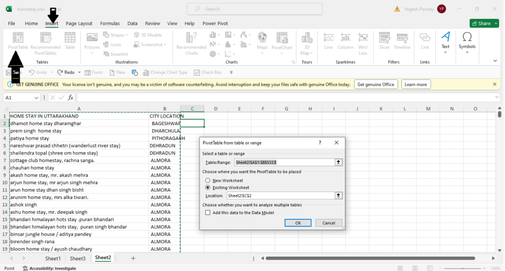
What is a PivotTable and how would you use it?

A PivotTable is a powerful tool in Excel used for summarizing, analyzing, and presenting large datasets in a more manageable and understandable format. It allows you to quickly analyze and extract insights from large amounts of data by summarizing it into a concise and interactive table.
Here’s how you can use a PivotTable in Excel:
1. Select Your Data: Start by selecting the dataset that you want to analyze. Make sure it’s organized with headers for each column.
2. Insert PivotTable: Go to the “Insert” tab on the ribbon and click on “PivotTable”. Excel will prompt you to select the range of data for the PivotTable and where you want to place it (either in a new worksheet or an existing one).
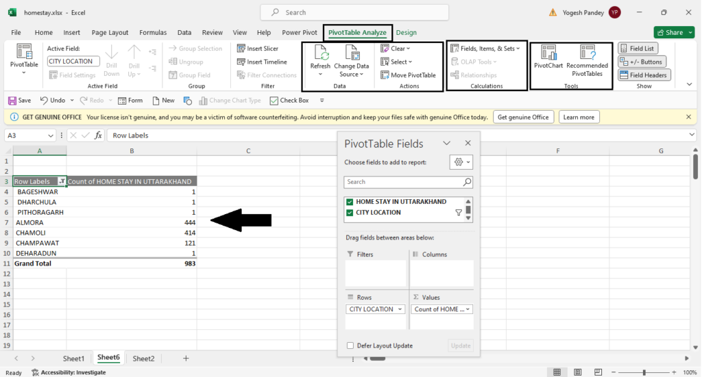
3. Design Your PivotTable: In the PivotTable Field List pane that appears on the right, you’ll see all the column headers from your dataset. Drag and drop the fields you want to analyze into the “Rows”, “Columns”, and “Values” areas of the PivotTable Field List to design your PivotTable.
4. Analyze Data: Once you’ve set up your PivotTable, Excel will automatically summarize your data based on the fields you’ve chosen. You can customize the summary by applying functions like sum, count, average, etc., to the values in the PivotTable.
5. Filter and Sort: You can easily filter and sort your data within the PivotTable to focus on specific subsets or trends within your dataset.
6. Refresh Data: If your original dataset changes, you can refresh the PivotTable to reflect the updated data. Right-click on the PivotTable and select “Refresh”.
7. Format and Customize: You can format the PivotTable to make it visually appealing and easier to understand. You can also customize the layout and appearance of the PivotTable using Excel’s formatting options.
Overall, PivotTables are incredibly useful for quickly summarizing and analyzing large datasets, identifying trends and patterns, and gaining valuable insights from your data.

What are some common data types in Excel?

In Excel, there are several common data types that are frequently used to store different kinds of information. Some of the common data types in Excel include:
Number: Used to store numerical values, including integers, decimals, and currency values.
Text/String: Used to store alphanumeric characters, text, and strings of characters.
Date: Used to store dates and times.
Boolean: Used to store logical values, such as TRUE or FALSE.
Error: Used to indicate errors in calculations or functions.
Formula: Used to store formulas that perform calculations based on other cell values.
Array: Used to store arrays or ranges of values.
These data types are fundamental to organizing and analyzing data in Excel and are used extensively in creating spreadsheets and performing various calculations and analyses.

What is the purpose of the INDIRECT function in Excel?

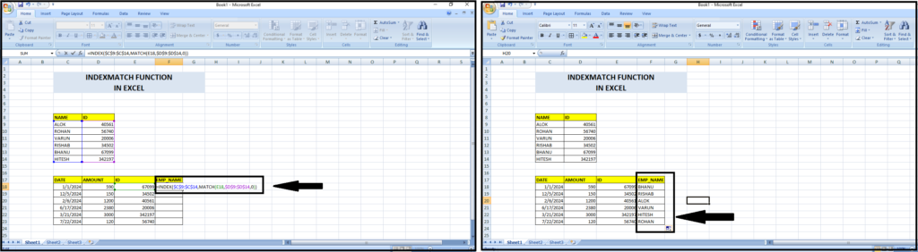
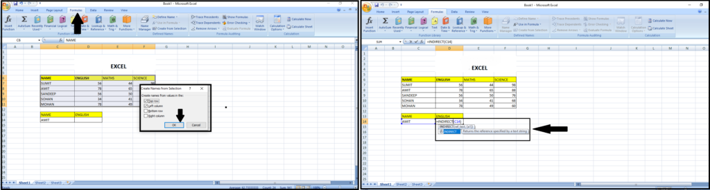
The INDIRECT function in Excel is used to convert a text string into a cell reference or range reference. Its primary purpose is to allow users to create dynamic references to cells or ranges based on the contents of other cells.

Syntax: INDIRECT(ref_text, [a1])

ref_text: The text string representing the cell reference or range reference.
[a1]: Optional. A logical value that specifies the reference style to use: TRUE (default) for A1-style reference or FALSE for R1C1-style reference.

The INDIRECT function is particularly useful in scenarios where you need to dynamically refer to different cells or ranges based on changing criteria or conditions. It allows for the creation of dynamic formulas and data manipulation techniques such as data validation, conditional formatting, and lookup functions.

For example, you can use INDIRECT to create a dynamic lookup formula that refers to a different table based on the selection made in another cell. Or, you can use it to dynamically refer to cells in different worksheets or workbooks based on specific criteria.

How would you calculate the percentage change between two values in Excel?

To calculate the percentage change between two values in Excel, you can use the following formula:

Here’s how you can implement it in Excel:

Subtract the old value from the new value.
Divide the result by the old value.
Multiply the result by 100 to convert it to a percentage.

In Excel, the formula would look like this:

For example, if the old value is in cell A1 and the new value is in cell A2, the formula in Excel would be:

$(A 1- A 2/ A 1) \times 100$

This formula will calculate the percentage change between the two values and display the result as a percentage.

How do you remove duplicate values in Excel?

To remove duplicate values in Excel, you can use the “Remove Duplicates” feature. Here’s how:
Select the Data Range: Click on any cell within the range of data from which you want to remove duplicates.
Open the Remove Duplicates Dialog Box: Go to the “Data” tab on the ribbon and click on “Remove Duplicates” in the Data Tools group. Excel will display a dialog box.
Choose Columns: In the Remove Duplicates dialog box, Excel will automatically select all columns. If you only want to remove duplicates based on specific columns, uncheck the columns you don’t want to include in the process.
Remove Duplicates: Once you’ve selected the columns, click “OK”. Excel will then remove any duplicate values from the selected range of data.
Confirmation: Excel will display a message indicating how many duplicate values were removed and how many unique values remain.
By following these steps, you can quickly remove duplicate values from your dataset in Excel. It’s important to note that the Remove Duplicates feature permanently deletes duplicate values from your data, so make sure to double-check before proceeding.

How would you sort data in Excel?

To sort data in Excel, you can use the built-in sorting functionality. Here’s how:
Select the Data Range: Click on any cell within the range of data you want to sort.
Open the Sort Dialog Box: Go to the “Data” tab on the ribbon, then click on “Sort” in the Sort & Filter group. Alternatively, you can right-click on any cell within the data range and choose “Sort” from the context menu.
Choose Sorting Options: In the Sort dialog box, you can specify the sorting options:
Select the column you want to sort by from the “Sort by” dropdown list.
Choose whether to sort in ascending or descending order using the options provided.
Optionally, you can add additional levels of sorting by clicking on the “Add Level” button and specifying further sorting criteria.
Apply Sorting: Once you’ve configured the sorting options, click “OK” to apply the sorting. Excel will rearrange the data according to the specified sorting criteria.
Alternatively, you can use the sorting buttons in the Excel toolbar to sort data quickly. These buttons are located in the “Home” tab, under the “Editing” group, and allow you to sort data in ascending or descending order based on the currently selected column.
By following these steps, you can easily sort data in Excel to organize it according to your preferences.