Power BI Data Modeling Guide with Examples & 50+ DAX Formulas

🚀 Power BI Data Modeling: The Foundation of Business Analytics

Table of Contents

Power BI is not just about creating dashboards—it’s about building a solid data model that delivers accurate, scalable, and meaningful insights. In simple words, Data Modeling in Power BI means:

📊 Connect Tables

Combine Sales, Customer, Product, and Date tables into one model.

🔗 Define Relationships

Link CustomerID & ProductID to analyze data seamlessly.

🧮 Use DAX Formulas

Calculate KPIs like Total Sales, Profit, and Customer Insights.

📂 Practice with Our Dataset

We’ve prepared a sample dataset with Sales, Customer, and Product tables for you. Download it and follow along with this guide.

👉 Download Dataset

🔹 How to Load This File into Power BI

Click the Download Dataset button above.
Go to File → Download → Microsoft Excel (.xlsx) in Google Sheets.
Open Power BI Desktop → Home → Get Data → Excel.
Select the file and load the tables (Sales, Customer, Product).
Go to Model View in Power BI → You’ll see all tables ready for relationships.

📊 Section 2: Understanding the Dataset (Sales, Customer & Product)

Before creating relationships and writing DAX formulas, you need to know what data you are working with. In this guide, we are using three key tables that form the foundation of our Power BI Data Model.

🛒 Sales Table (Fact Table)

Contains all transaction-level details such as Order Date, Customer, Product, Quantity, Sales Amount, Profit, Discount, Region, and Payment Method. This is our Fact Table where all measures like Total Sales, Total Profit, and Orders Count will be calculated.

OrderID – Unique order number
OrderDate – Date of order
CustomerID, ProductID – Keys to connect with Customer & Product tables
SalesAmount, Profit, Quantity, Discount
Region, City, State, SalesChannel

👤 Customer Table (Dimension Table)

Stores detailed customer information including demographics, region, and engagement. This is a Dimension Table used for slicing and dicing the Sales data.

CustomerID – Primary Key (links to Sales table)
CustomerName, Gender, Age, AgeGroup
Region, City, State, Country
LoyaltyPoints, Membership, SatisfactionScore
ChurnRisk, LastPurchaseDate

📦 Product Table (Dimension Table)

Contains details of products sold including category, sub-category, supplier, and cost information. This is another Dimension Table that helps analyze Sales by product attributes.

ProductID – Primary Key (links to Sales table)
ProductName, Category, SubCategory
Brand, SupplierName, CountryOfOrigin
Price, Cost, Profitability
StockQuantity, Warranty, ReturnRate

📌 Note:

Together, these tables form a Star Schema in Power BI. The Sales table acts as the central fact table, while Customer and Product tables act as dimensions. This design ensures faster queries, simplified DAX formulas, and scalable analytics.

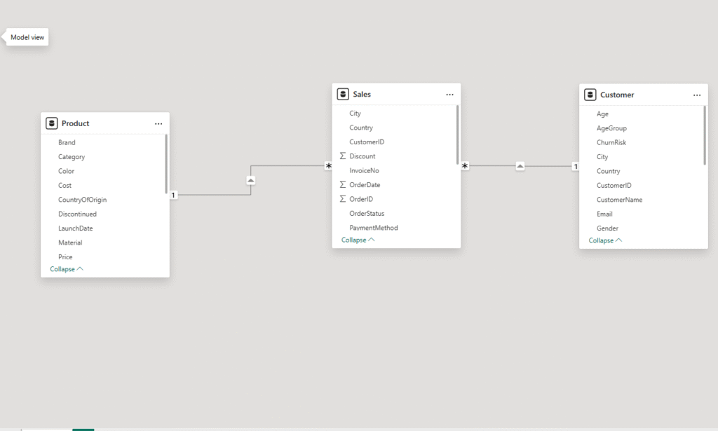
⭐ Section 3: Building a Star Schema in Power BI

Once we load our dataset into Power BI, the next step is to create a Star Schema. A Star Schema keeps one Fact Table (Sales) at the center and multiple Dimension Tables (Customer, Product, Date) connected around it. This design makes your model simple, efficient, and easy to query.

📌 Diagram Here

Sales (Fact) → Customer (Dim), Product (Dim), Date (Dim)

(Insert Star Schema image in your WordPress/Elementor editor)

🔗 Step 1: Create Relationships

Sales[CustomerID] → Customer[CustomerID] (One-to-Many)
Sales[ProductID] → Product[ProductID] (One-to-Many)
Sales[OrderDate] → Date[Date] (One-to-Many)

👉 Make sure cross-filter direction is set to Single for best performance.

📐 Step 2: Understand Cardinality

Cardinality defines how tables are related. In our case:

1 → Many: One Customer can have many Sales orders.
1 → Many: One Product can appear in many Sales orders.
1 → Many: One Date can link to multiple Sales orders.

✨ Why Use a Star Schema?

✔️ Easy to understand for both developers and business users
✔️ Optimized for faster queries and DAX calculations
✔️ Reduces complexity compared to snowflake schemas
✔️ Makes adding KPIs & visuals straightforward

📅 Section 4: Adding a Date Table for Time Intelligence

Time-based analysis is one of the most important aspects of Business Analytics. To enable calculations like YTD (Year-to-Date), MTD (Month-to-Date), QTD (Quarter-to-Date) or Previous Year Sales, you must create a dedicated Date Table in Power BI.

📌 Why Do We Need a Date Table?

✔️ Required for all Time Intelligence DAX Functions
✔️ Provides consistent Year, Quarter, Month breakdowns
✔️ Helps build Date Hierarchies (Year → Month → Day)
✔️ Makes trend analysis & forecasting easier

🧮 DAX Formula to Create a Date Table

Date = CALENDAR (DATE(2023,1,1), DATE(2023,12,31))

This formula creates a Date Table from 1st Jan 2023 to 31st Dec 2023. You can adjust the date range as per your dataset.

➕ Add Extra Columns for Analysis

Year    = YEAR('Date'[Date])
Month   = FORMAT('Date'[Date], "MMMM")
Quarter = "Q" & FORMAT('Date'[Date], "Q")
Weekday = FORMAT('Date'[Date], "DDD")

These columns will allow you to build flexible reports such as Sales by Year, Sales by Quarter, Sales by Month, and Sales by Weekday.

📝 Step-by-Step: How to Create & Use the Date Table

Go to Modeling → New Table in Power BI Desktop.
Paste the DAX formula Date = CALENDAR (DATE(2023,1,1), DATE(2023,12,31)).
Power BI will generate a new table named Date.
Add calculated columns (Year, Month, Quarter, Weekday) for hierarchy.
Go to Model View → Right click Date Table → Mark as Date Table.
Connect Sales[OrderDate] with Date[Date] to enable time intelligence.
Now you can use formulas like Sales YTD, Sales MTD, Previous Year Sales.

🧮 Section 5: Calculated Columns vs Measures in Power BI

One of the most common questions in Power BI is: When should I use a Calculated Column, and when should I use a Measure? Let’s break this down with simple examples and pros & cons.

📌 Calculated Columns

A Calculated Column is created at the row level in your table. It adds a new column to the dataset and stores values for each row.

Profit Margin Column = Sales[Profit] / Sales[SalesAmount]

Use Cases: Categorization, grouping, flags (e.g., High/Low Sales, Age Groups).

✔️ Stored in the table (persistent)
✔️ Can be used in relationships
❌ Increases data model size
❌ Slower if overused

📌 Measures

A Measure is a calculation performed on demand (in memory) and does not create a physical column in the table.

Total Sales = SUM(Sales[SalesAmount])

Use Cases: Aggregations like totals, averages, ratios, percentages.

✔️ Lightweight, efficient
✔️ Faster performance
✔️ Best for KPIs and visuals
❌ Cannot be used in relationships

⚖️ Key Difference

👉 Calculated Columns = Row-level calculations (stored in the model)
👉 Measures = Aggregated calculations (calculated on demand)

✅ Best Practice: Use Measures for KPIs and reports, and Calculated Columns only when absolutely necessary.

🧮 Section 6: 50+ DAX Formulas for Business Analytics

Here are 50+ practical DAX formulas grouped into categories. Each formula also mentions the table where it is applied (Sales, Customer, Product, Date). These are the must-know formulas for every Business Analyst.

📝 How to Create a DAX Formula in Power BI

Open Power BI Desktop.
Go to Modeling → New Measure (or New Column for row-level calculations).
Enter the DAX formula (see examples below).
Press Enter → The new measure will appear under the respective table.
Drag & drop the measure into a visual (Card, Table, Chart) to see results.

📊 A. Basic KPIs (Sales Table)

Total Sales (Sales Table)    = SUM(Sales[SalesAmount])
Total Profit (Sales Table)   = SUM(Sales[Profit])
Orders Count (Sales Table)   = DISTINCTCOUNT(Sales[OrderID])
Average Sales (Sales Table)  = AVERAGE(Sales[SalesAmount])

Role: Core KPIs for revenue, profit, and transaction volume.

⏳ B. Time Intelligence (Date + Sales Tables)

Sales YTD (Date + Sales)       = TOTALYTD([Total Sales], 'Date'[Date])
Sales MTD (Date + Sales)       = TOTALMTD([Total Sales], 'Date'[Date])
Previous Year Sales (Date)     = CALCULATE([Total Sales], SAMEPERIODLASTYEAR('Date'[Date]))
Sales Growth % (Date + Sales)  = DIVIDE([Total Sales]-[Previous Year Sales],[Previous Year Sales],0)

Role: Enables YTD, MTD, and year-over-year comparisons.

👥 C. Customer Insights (Customer + Sales Tables)

Unique Customers (Sales)          = DISTINCTCOUNT(Sales[CustomerID])
Avg Sales per Customer (Sales)    = DIVIDE([Total Sales], [Unique Customers], 0)
Platinum Customers (Customer)     = CALCULATE([Total Sales], Customer[Membership]="Platinum")
High Churn Risk Sales (Customer)  = CALCULATE([Total Sales], Customer[ChurnRisk]="High")

Role: Helps identify loyalty segments and customer retention risks.

📦 D. Product Performance (Product + Sales Tables)

Profit Margin % (Sales)    = DIVIDE([Total Profit], [Total Sales], 0)
Top Product (Product)      = RANKX(ALL(Product), [Total Sales],,DESC)
Stock Value (Product)      = SUMX(Product, Product[StockQuantity]*Product[Price])
Return Impact (Sales)      = SUMX(FILTER(Sales, Sales[ReturnFlag]=1), Sales[SalesAmount])

Role: Evaluates product performance, inventory value, and returns impact.

🌍 E. Regional & Channel Analysis (Sales Table)

Sales by Region (Sales)   = CALCULATE([Total Sales], ALLEXCEPT(Sales, Sales[Region]))
Online Sales (Sales)      = CALCULATE([Total Sales], Sales[SalesChannel]="Online")
Retail Sales (Sales)      = CALCULATE([Total Sales], Sales[SalesChannel]="Retail Store")
Profit by City (Sales)    = SUMMARIZE(Sales, Sales[City], "Profit", [Total Profit])

Role: Analyzes performance across regions, cities, and sales channels.

💰 F. Financial Metrics (Sales Table)

Gross Profit (Sales)        = [Total Sales] - SUM(Sales[ShippingCost])
Operating Profit (Sales)    = [Gross Profit] - SUM(Sales[Discount])
Avg Order Value (Sales)     = DIVIDE([Total Sales], [Orders Count], 0)
Customer Lifetime Val (Cust)= [Avg Sales per Customer] * 12

Role: Measures financial efficiency: margins, profitability, and CLV.

📈 G. Advanced Analytics (Date + Sales + Product)

Moving Average 3M (Date+Sales) = AVERAGEX(DATESINPERIOD('Date'[Date], MAX('Date'[Date]), -3, MONTH), [Total Sales])
Cumulative Sales (Date+Sales)  = CALCULATE([Total Sales], FILTER(ALL('Date'), 'Date'[Date]<=MAX('Date'[Date])))
% of Total Sales (Sales)       = DIVIDE([Total Sales], CALCULATE([Total Sales], ALL(Sales)))
Market Share Cat (Product)     = DIVIDE([Sales by Category], CALCULATE([Total Sales], ALL(Product)))

Role: Enables forecasting, cumulative trends, and market share analysis.

🎯 Final Role of These Formulas

These 50+ DAX formulas span across Sales, Customer, Product, and Date tables. They power dashboards for:

✔️ Sales KPIs – Revenue, Profit, Growth
✔️ Customer Insights – Loyalty, Churn, Lifetime Value
✔️ Product Analysis – Top Products, Inventory, Returns
✔️ Regional Trends – Channel & Location Performance
✔️ Financial Health – Margins & Profitability
✔️ Advanced Analytics – Forecasting & Trend Analysis

This is exactly what a Business Analyst needs in real-world projects.

✅ Section 7: Best Practices for Power BI Data Modeling

A great Power BI report is built on a well-structured data model. Follow these best practices to ensure your dashboards are accurate, fast, and easy to maintain.

⭐ Use Star Schema

Keep Fact Tables (Sales) at the center.
Connect with Dimension Tables (Customer, Product, Date).
Reduces complexity vs Snowflake schema.

🧮 Prefer Measures over Columns

Measures are faster and memory-efficient.
Use Calculated Columns only when necessary.
Example: Use a Total Sales measure instead of column aggregation.

📅 Always Create a Date Table

Required for Time Intelligence (YTD, MTD, QTD).
Mark it as Date Table in Power BI.
Enables hierarchies: Year → Quarter → Month → Day.

👁️ Hide Unnecessary Columns

Keep model clean & user-friendly.
Hide keys (like CustomerID, ProductID) from report view.
Expose only business-friendly fields.

🔗 Manage Relationships Carefully

Use Single direction filtering for performance.
Avoid unnecessary bi-directional relationships.
Check Cardinality (1:1, 1:M) before linking.

⚡ Optimize for Performance

Reduce Calculated Columns, prefer Measures.
Import only necessary fields from source.
Use aggregations for large datasets.

💡 Pro Tips for Analysts

✔️ Name measures clearly (e.g., Total Sales, Profit Margin %).
✔️ Group related measures into folders in Power BI for easy access.
✔️ Document your model (tables, keys, measures) for teamwork.
✔️ Always validate results by cross-checking with raw data.

🧩 Section 7B: Data Modeling Functions Toolkit

Beyond schema design, Power BI offers DAX functions that directly support data modeling. These functions let you pull related values, activate relationships, and even create virtual joins. Let’s explore them in detail with examples from our Sales, Customer, Product, and Date tables.

🔗 RELATED()

Customer Region = RELATED(Customer[Region])

What it does: Pulls a column value from a related Dimension table into the Fact table. Example: From the Customer table, fetch Region into the Sales table.

Business Role: Useful when you need Customer or Product details in the Sales table for easier reporting. (Excel users can think of this as VLOOKUP in DAX).

📑 RELATEDTABLE()

Customer Orders = COUNTROWS(RELATEDTABLE(Sales))

What it does: Returns all rows from a related table for the current row context. Example: In the Customer table, count how many orders each customer placed in the Sales table.

Business Role: Helps create Customer KPIs → “Number of Orders per Customer”.

🛠 USERELATIONSHIP()

Sales by Ship Date = CALCULATE([Total Sales], USERELATIONSHIP(Sales[ShipDate], Date[Date]))

What it does: Activates an inactive relationship for a calculation. Example: Use ShipDate instead of OrderDate to calculate Total Sales.

Business Role: Perfect for businesses that track multiple dates: Order Date, Ship Date, Invoice Date.

🔄 CROSSFILTER()

Sales Both Direction = CALCULATE([Total Sales], CROSSFILTER(Customer[CustomerID], Sales[CustomerID], BOTH))

What it does: Temporarily overrides filter direction between two tables. Example: Apply bi-directional filtering between Customer and Sales for a calculation.

Business Role: Useful when slicers or filters need to flow in both directions (but should be used sparingly for performance).

🔍 LOOKUPVALUE()

Customer AgeGroup = LOOKUPVALUE(Customer[AgeGroup], Customer[CustomerID], Sales[CustomerID])

What it does: Returns a single value from another table, like Excel’s VLOOKUP. Example: Fetch AgeGroup from the Customer table into the Sales table.

Business Role: Good for quick lookups when you don’t want to create a relationship.

🎭 TREATAS()

Filter Sales = CALCULATE([Total Sales], TREATAS(VALUES(Product[Category]), Sales[ProductCategory]))

What it does: Applies values from one table as filters to another table → creates a virtual relationship. Example: Filter Sales data using Product categories even if there is no direct relationship.

Business Role: Extremely powerful for complex models or “what-if” analysis.

📌 Final Note

These Data Modeling Functions give analysts fine control over relationships, lookups, and filters inside Power BI. By mastering them, you go beyond simple KPIs and build models that are smarter, more flexible, and closer to real business needs.

Power BI Data Modeling: Guide with Examples & 50+ DAX Formulas