
Master Probability in Data Science Complete 2026 Guide with Theory, Formulas, Python Examples and Real Projects | The Vista Academy Dehradun
Master Probability in Data Science – Theory • Formulas • Python • Machine Learning • Real Projects

Learn Probability from fundamentals to advanced Data Science applications with Python, Machine Learning, interview questions, and real-world projects.

Probability for Data Science • Introduction

Why Probability Is the Real Backbone of Data Science

Probability is the mathematical language behind every intelligent prediction made in Data Science, Machine Learning, Artificial Intelligence, and Business Analytics. Whether you’re building a recommendation engine, detecting fraud, forecasting sales, or training a predictive model, probability helps computers make decisions under uncertainty. In this complete guide, you’ll learn not only the theory of probability but also how it powers real-world data science applications using Python.

Ask ten experienced data scientists which mathematical concept they rely on almost every day, and most will answer with a single word—Probability.

While Python, SQL, Power BI, and Machine Learning libraries receive most of the attention, probability is the invisible engine working behind every prediction, recommendation, classification, and forecast. It is the foundation upon which modern Data Science is built.

When Netflix recommends your next movie, it is estimating the probability that you’ll enjoy watching it. When Amazon suggests products, it predicts the likelihood of a purchase. Banks evaluate the probability of loan default, hospitals estimate disease risk, insurance companies calculate claim probabilities, and spam filters determine whether an email belongs in your inbox or junk folder.

In simple words, every intelligent system makes decisions based on probabilities rather than certainty.

Without understanding probability, you’ll be able to write Machine Learning code—but you’ll struggle to explain why the algorithm works, how predictions are made, or how to improve model accuracy during real-world projects and interviews.

Why We Teach Probability First at The Vista Academy

At The Vista Academy, Dehradun, we believe probability isn’t just another mathematics chapter to memorize before learning Python or Machine Learning.

Instead, it is treated as the first building block of every Data Analytics and Data Science program because students who understand probability learn algorithms faster, interpret results more confidently, and perform significantly better during technical interviews.

Rather than memorizing formulas, our learners understand how probability influences classification models, regression algorithms, Bayesian learning, recommendation systems, A/B testing, predictive analytics, and AI decision-making.

Who Should Read This Guide?

Complete Beginners Start from absolute basics and understand whether Data Science is the right career path before diving into Python or Machine Learning.
Working Professionals Transition from finance, operations, engineering, marketing, or IT into Data Analytics, AI, and Data Science with a strong mathematical foundation.
College Students Build concepts that help you understand Machine Learning instead of simply copying code from online tutorials.
Interview Preparation Revise probability concepts commonly asked during Data Analyst, Data Scientist, Machine Learning, and Business Analyst interviews.

What You’ll Learn in This Complete Probability Guide

✔ Probability Fundamentals Sample Space, Events, Random Variables, Conditional Probability, Independence, and Bayes’ Theorem explained with intuitive examples.
✔ Mathematical Formulas Understand every important probability formula instead of memorizing it blindly.
✔ Python Programming Solve practical probability problems using NumPy, Pandas, SciPy, and Matplotlib with step-by-step Python examples.
✔ Real Data Science Projects See how probability powers fraud detection, recommendation engines, predictive analytics, A/B testing, forecasting, NLP, and Machine Learning models.

Why This Guide Is Different

Many online tutorials fall into one of two extremes. Some are filled with mathematical proofs but never explain how those formulas are used in Data Science. Others oversimplify concepts so much that learners know the terminology but cannot apply probability during projects or interviews.

This guide follows a practical learning approach. Every concept begins with simple intuition, followed by mathematical understanding, Python implementation, interview insights, and finally a real-world Data Science application.

This mirrors the same learning methodology used at The Vista Academy, where every theoretical concept is immediately connected to hands-on coding, analytics projects, and business case studies.

Our objective is simple: by the time you complete this guide, you won’t just know probability—you’ll understand how Data Scientists actually use it to solve real business problems.

Probability concepts and formulas used in data science explained by The Vista Academy Dehradun
Master Probability for Data Science with Python, Machine Learning & Real Projects
Section 1 • Probability Basics

What Exactly Is Probability? (Definitions Every Data Science Beginner Must Know)

Probability is one of the most important concepts in Data Science, Machine Learning, Artificial Intelligence, Statistics, and Business Analytics. Every prediction made by a machine learning model is based on probability. Before learning algorithms like Linear Regression, Decision Trees, or Neural Networks, it’s essential to understand what probability actually means.

What Is Probability?

In simple words, probability measures how likely an event is to happen. It is represented by a number between 0 and 1.

Think of probability as a confidence score. The closer the value is to 1, the more likely the event will happen. The closer it is to 0, the less likely it is to occur.

Probability = 0 The event is impossible.

Example: Rolling a 7 on a standard six-sided dice.
Probability = 1 The event is certain.

Example: A six-sided dice will always land on a number between 1 and 6.
Probability = 0.5 The event has an equal chance of happening or not happening.

Example: Getting Heads when tossing a fair coin.

The Classical Probability Formula

For simple situations like coins, dice, and playing cards, probability is calculated using the classical formula:

Probability Formula P(Event) = Number of Favourable Outcomes ÷ Total Number of Possible Outcomes

Example 1: Rolling a Dice

Suppose you roll a fair six-sided dice and want to know the probability of getting the number 4.

Total Possible Outcomes 1, 2, 3, 4, 5, 6

Total = 6
Favourable Outcomes Only one outcome satisfies the condition:

{4}
Probability P(4) = 1 ÷ 6 = 0.1667

There is approximately a 16.7% chance of rolling a 4.

Example 2: Real Data Science Example

Imagine an online shopping website where 10,000 visitors visited yesterday.

  • 10,000 people visited the website.
  • 800 customers purchased a product.

The probability that a randomly selected visitor made a purchase is:

Purchase Probability P(Buy) = 800 ÷ 10,000 = 0.08 This means there is an 8% probability that a new visitor will purchase a product.

This simple probability becomes the starting point for recommendation systems, customer segmentation, sales forecasting, and conversion prediction models used by companies like Amazon, Flipkart, Netflix, and Google.

Classical Probability vs Empirical Probability

The classical formula works perfectly when every possible outcome is known beforehand—such as dice, cards, or coins.

However, in Data Science, we rarely work with perfect games. Instead, we analyze historical data to estimate probabilities.

Classical Probability Used for coins, dice, cards, and mathematical experiments where all outcomes are known.
Empirical Probability Estimated using historical data such as customer purchases, disease diagnosis, loan defaults, fraud detection, or website clicks.

For example, if historical banking data shows that 2 out of every 100 customers default on a loan, the bank estimates the probability of default using real data instead of mathematical assumptions.

Important Probability Terms Every Beginner Should Know

Experiment Any activity that produces an outcome.

Example: A customer visits an online shopping website.
Sample Space (S) The complete set of all possible outcomes.

Example: Buy or Doesn’t Buy.
Event (E) The particular outcome we want to measure.

Example: Customer buys a laptop.
Trial One repetition of the experiment.

Example: One customer visiting the website.

💡 Interview Tip: Most beginners jump directly into Machine Learning algorithms without understanding these four basic terms. Surprisingly, interviewers often ask these concepts because they form the foundation of Naive Bayes, Logistic Regression, Decision Trees, A/B Testing, and Predictive Analytics.

Why This Matters in Data Science

Every Machine Learning model predicts probabilities before making decisions.

  • Spam Detection → Probability an email is spam.
  • Loan Approval → Probability a customer will default.
  • Medical Diagnosis → Probability a patient has a disease.
  • Netflix Recommendation → Probability you’ll watch a movie.
  • Customer Churn → Probability a customer will leave a company.

Once you understand these basic probability concepts, advanced topics like Conditional Probability, Bayes’ Theorem, Probability Distributions, and Machine Learning Algorithms become much easier to understand.

Probability concepts explained for Data Science beginners with real-world examples by The Vista Academy Dehradun
Probability Basics for Data Science • Learn with Real Examples
Section 2 • Probability in Data Science

Why Data Scientists Cannot Avoid Probability

Every successful Data Scientist works with uncertainty. Customers may or may not buy a product, a patient may or may not have a disease, and a loan applicant may or may not default. Probability is the mathematical framework that helps transform this uncertainty into informed, data-driven decisions. That’s why probability is considered one of the core foundations of Data Science, Machine Learning, Artificial Intelligence, Predictive Analytics, and Business Intelligence.

Can You Learn Data Science Without Probability?

One of the most common questions we hear at The Vista Academy, Dehradun is:

“Sir, I only want to learn Python and Power BI. Can I skip probability?”

The practical answer is partially yes—but only up to a point.

If your goal is creating dashboards, reports, and data visualizations, basic statistics may be enough. However, the moment you move into Machine Learning, Artificial Intelligence, Predictive Analytics, Recommendation Systems, or Data Science interviews, probability becomes unavoidable.

Every predictive model estimates the likelihood of an event occurring before making a decision.

Where Probability Is Used in Data Science

📊 Model Evaluation Metrics such as Precision, Recall, ROC Curve, AUC, F1-Score, and prediction confidence are directly connected to probability.
🤖 Machine Learning Algorithms Algorithms like Naive Bayes, Logistic Regression, Hidden Markov Models, Bayesian Networks, and Gaussian Models rely heavily on probability theory.
🧪 A/B Testing Companies determine whether a new website design or marketing campaign genuinely improves conversions—or whether the difference happened by chance.
💳 Banking & Risk Analysis Banks estimate the probability that customers will repay loans, default on credit cards, or become high-risk borrowers.
💬 Natural Language Processing (NLP) Chatbots, voice assistants, translators, and autocomplete systems predict the next word using probability distributions.
🎬 Recommendation Systems Netflix, YouTube, Spotify, and Amazon recommend content by estimating the probability that you’ll click, watch, or purchase.
🚨 Fraud & Anomaly Detection Unusual transactions with extremely low probability are automatically flagged as suspicious or fraudulent.
📈 Sales Forecasting Businesses estimate future sales, customer demand, inventory needs, and market trends using probabilistic models.

Real-World Example

Imagine an online payment company processes 1 million transactions every day.

Normally, only 0.05% of these transactions are fraudulent.

When a new transaction arrives, the Machine Learning model doesn’t simply label it as “Fraud” or “Safe.”

Instead, it calculates something like:

Fraud Prediction Probability(Transaction is Fraud) = 97.8% Since this probability is extremely high, the system automatically blocks the payment and asks for additional verification.

This is exactly how probability powers fraud detection systems used by banks, payment gateways, and fintech companies around the world.

Examples You Use Every Day

Netflix Predicts the probability that you’ll enjoy a movie before recommending it.
Google Maps Estimates the probability of traffic congestion and predicts your arrival time.
Gmail Calculates the probability that an incoming email is spam.
Amazon Ranks products according to the probability you’ll purchase them.
Healthcare AI Predicts the probability of diseases using patient symptoms and medical history.
Weather Forecasting When the forecast says “80% chance of rain,” that’s a probability prediction generated from historical and real-time weather data.

💡 Interview Insight: Recruiters often ask candidates to explain how Logistic Regression predicts customer churn or how Naive Bayes detects spam emails. Both questions fundamentally test your understanding of probability—not your ability to memorize Python syntax.

The Bottom Line

Probability is not just another chapter in mathematics—it is the language of uncertainty. Every Machine Learning model, AI application, predictive algorithm, recommendation engine, and risk analysis system uses probability to make intelligent decisions.

Once you understand probability, advanced topics such as Bayes’ Theorem, Probability Distributions, Statistical Inference, Hypothesis Testing, and Machine Learning Algorithms become significantly easier to learn.
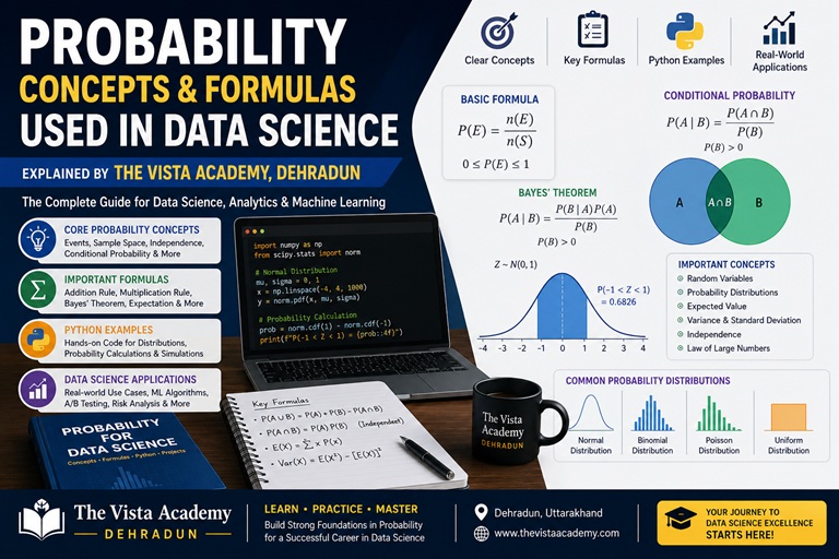
Probability concepts and formulas used in data science explained by The Vista Academy Dehradun
Probability Powers Machine Learning, AI & Predictive Analytics

Discover how probability is used in Machine Learning, Artificial Intelligence, fraud detection, recommendation systems, A/B testing, and predictive analytics.

Section 3 • Types of Probability

Types of Probability in Data Science: Classical, Empirical & Subjective

Not every probability is calculated in the same way. Sometimes we know all possible outcomes, sometimes we learn from historical data, and sometimes we rely on expert judgment. Understanding these three types of probability helps Data Scientists choose the right approach for solving real-world business problems.

Why Do We Need Different Types of Probability?

Imagine you are asked three completely different questions:

🎲 Question 1 What is the probability of rolling a 4 on a fair dice?
🛒 Question 2 What is the probability that a website visitor will purchase a product?
🏦 Question 3 What is the probability that a brand-new startup will succeed?

Although all three questions ask about probability, they cannot be solved using the same method.

That’s why probability is divided into three major types.

1. Classical (Theoretical) Probability

Classical Probability is used when every possible outcome has an equal chance of occurring. Since all outcomes are equally likely, we can calculate probability using a simple mathematical formula.

Formula Probability = Favourable Outcomes ÷ Total Possible Outcomes

🎲 Example: Rolling a Dice

A fair dice has six sides.

Possible outcomes are: 1, 2, 3, 4, 5, 6

If you want to know the probability of getting a 4:

Calculation Favourable Outcomes = 1
Total Outcomes = 6

P(4) = 1/6 = 0.1667

This means there is a 16.67% chance of rolling a 4.

💡 Classical probability is mainly used in mathematics, games, cards, coins, lotteries, and simple probability problems.

2. Empirical (Experimental) Probability

Empirical Probability is calculated using real historical data instead of assumptions.

This is the type of probability that Data Scientists use most often because business data rarely has equally likely outcomes.

Instead of asking, “What should happen?” we ask, “What actually happened in the past?”

🛒 Example: Online Shopping Website

Suppose an e-commerce website received:

  • 40,000 visitors last month
  • 3,200 customers purchased a product
Calculation Probability of Purchase

= 3200 ÷ 40000

= 0.08

=8%

This means that, based on historical data, a randomly selected visitor has approximately an 8% probability of making a purchase.

📊 Where Is It Used?

Customer Churn Prediction Estimate how likely customers are to leave a company.
Fraud Detection Predict whether a transaction is fraudulent.
Sales Forecasting Estimate future product demand.
Recommendation Systems Predict what customers are most likely to purchase or watch.

⭐ If you’re learning Data Science, this is the probability you’ll use more than 90% of the time.

3. Subjective Probability

Sometimes there isn’t enough historical data to calculate probability mathematically.

In such situations, experts use their experience, knowledge, intuition, and judgment to estimate probability.

This is called Subjective Probability.

🏦 Example: Loan Approval

A startup company applies for a loan.

Since the company is new, there is very little historical data available.

An experienced loan officer reviews:

  • Business plan
  • Founder’s experience
  • Market demand
  • Cash flow
  • Industry growth

Based on experience, the officer says:

Expert Judgment “I believe this company has around a 70% chance of repaying the loan.”

Notice that this probability wasn’t calculated using a formula—it was estimated using professional experience.

Modern Bayesian Machine Learning combines expert knowledge with historical data to continuously improve these estimates as new information becomes available.

Quick Comparison

🎲 Classical Probability Used when all outcomes are equally likely.

Example: Dice, Coins, Cards.
📊 Empirical Probability Calculated using historical observations.

Example: Customer purchases, Loan defaults, Sales data.
🧠 Subjective Probability Estimated using expert judgment and experience.

Example: Business success, Startup investment, Medical diagnosis.
Section 4 • Probability Rules

The Fundamental Rules of Probability Every Data Scientist Should Know

Before learning Bayes’ Theorem, Probability Distributions, Machine Learning Algorithms, or Hypothesis Testing, you must understand the basic rules of probability. These simple rules are used repeatedly in Data Science, Business Analytics, Artificial Intelligence, and Statistics. Once you master them, advanced probability becomes much easier to understand.

Why Are Probability Rules Important?

Imagine you’re building a Machine Learning model to predict customer behavior.

The model may need to answer questions like:

🛒 Customer Analytics What is the probability that a customer buys a laptop or a smartphone?
🏦 Banking What is the probability that a customer defaults on a loan or misses an EMI payment?
🏥 Healthcare What is the probability that a patient has fever or cough?

To answer these kinds of questions correctly, Data Scientists use the Addition Rule of Probability.

4.1 The Addition Rule (OR Rule)

The Addition Rule is used whenever we want to calculate the probability that Event A OR Event B happens.

Formula P(A OR B) = P(A) + P(B) − P(A AND B)

Notice the last part of the formula: P(A AND B).

Why do we subtract it?

Because if an outcome belongs to both Event A and Event B, we accidentally count it twice when adding P(A) and P(B). Subtracting the overlap removes this duplicate counting.

💡 Think of it like counting students in two clubs. If some students belong to both clubs, you shouldn’t count those students twice.

Easy Example: Customer Database

Suppose a company has a customer database containing 1,000 customers.

The marketing team wants to know:

“What is the probability that a randomly selected customer is from Delhi OR Dehradun?”

After analyzing the data, they find:

Delhi Customers 300 customers live in Delhi.
Dehradun Customers 200 customers live in Dehradun.
Total Customers 1000 customers.

Now convert these numbers into probabilities:

  • Probability(Customer is from Delhi) = 300 ÷ 1000 = 0.30
  • Probability(Customer is from Dehradun) = 200 ÷ 1000 = 0.20

Also assume that every customer has only one address.

That means:

No Overlap A customer cannot live in both Delhi and Dehradun at the same time.

Therefore, P(Delhi AND Dehradun) = 0

Now apply the Addition Rule:

Calculation P(Delhi OR Dehradun)

= 0.30 + 0.20 − 0

=0.50

This means there is a 50% probability that a randomly selected customer belongs to either Delhi or Dehradun.

Why Do We Sometimes Subtract the Overlap?

Let’s look at another situation.

Suppose instead of cities, we study customers who purchased products.

  • 40% purchased a Laptop.
  • 35% purchased a Smartphone.
  • 15% purchased both Laptop and Smartphone.

If we simply add:

Wrong Calculation 40% + 35% = 75%

The problem is that customers who bought both products are counted twice.

To fix this, subtract the overlap:

Correct Calculation P(Laptop OR Smartphone)

= 0.40 + 0.35 − 0.15

=0.60

The correct probability is 60%, not 75%.

💡 This “subtract the overlap” idea is used everywhere in Data Science—from customer segmentation and recommendation systems to fraud detection and marketing analytics.

Special Case: Mutually Exclusive Events

Two events are called Mutually Exclusive when they cannot happen at the same time.

Examples include:

🎲 Dice A dice cannot show both 2 and 5 in a single roll.
🌆 Cities A customer cannot permanently live in Delhi and Dehradun simultaneously.
🚦Traffic Signal A traffic light cannot be both Red and Green at exactly the same moment.

For mutually exclusive events:

Simplified Formula P(A OR B) = P(A) + P(B)

4.2 The Multiplication Rule (AND Rule)

While the Addition Rule helps us calculate the probability of Event A OR Event B, the Multiplication Rule is used when we want both events to happen together.

In simple words, if your question contains the word “AND”, you will often use the Multiplication Rule.

Formula (Independent Events) P(A AND B) = P(A) × P(B)

💡 This formula only works when the two events are independent, meaning one event does not change the probability of the other.

Easy Example: Website Visitors

Suppose an e-commerce company analyzes 10,000 website visitors.

  • 70% of visitors are from India.
  • 65% of visitors use a mobile phone.

The marketing team wants to estimate:

What is the probability that a visitor is from India AND uses a mobile phone?

Assuming these two events are independent, we simply multiply the probabilities.

Calculation P(India AND Mobile)

= 0.70 × 0.65

=0.455

=45.5%

This means that approximately 4,550 out of every 10,000 visitors are expected to be both from India and using a mobile device.

📊 Data Scientists use this rule in customer segmentation, marketing analytics, recommendation systems, fraud detection, and predictive modeling.

However, if being from India actually influences whether someone uses a mobile device, then the events are not independent. In that case, we cannot simply multiply the probabilities—we must use Conditional Probability, which you’ll learn in the next section.

4.3 The Complement Rule (NOT Rule)

Sometimes it’s much easier to calculate the probability that an event does not happen rather than the probability that it does happen.

This is where the Complement Rule becomes useful.

Formula P(Not A) = 1 − P(A)

Example: Spam Email Detection

Suppose a Machine Learning model correctly identifies spam emails 92% of the time.

The probability of correctly detecting spam is:

P(Correct) = 0.92

What is the probability that the model makes a mistake?

Calculation P(Wrong)

= 1 − 0.92

=0.08

=8%

So, the spam detection model has an 8% probability of misclassifying an email.

🤖 The Complement Rule is widely used in Machine Learning, Quality Control, Medical Diagnosis, Fraud Detection, and Risk Analysis.

4.4 Mutually Exclusive vs Independent Events (A Common Beginner Confusion)

Many beginners think Mutually Exclusive and Independent mean the same thing.

They do not.

Understanding the difference is extremely important because using the wrong probability rule can produce completely incorrect results.

🚫 Mutually Exclusive Events Both events cannot happen together.

Example: A single coin toss cannot be both Heads and Tails at the same time.
✅ Independent Events Both events can happen together, but one event does not affect the probability of the other.

Example: Today’s weather in Dehradun and today’s stock market movement are unrelated.

Another Easy Example

Mutually Exclusive Rolling a dice: You cannot roll both 2 and 5 in one throw. Only one outcome is possible.
Independent Flip a coin and roll a dice. Whether the coin lands Heads or Tails does not affect the number shown on the dice. Both events happen independently.

🎯 Remember this shortcut:

Mutually Exclusive → Cannot happen together.
Independent → Can happen together, but one does not influence the other.

This distinction becomes extremely important in Machine Learning, Feature Engineering, Bayesian Statistics, Predictive Analytics, and A/B Testing. Many interview questions are designed specifically to test whether candidates understand this difference.

4.5 Practice Questions: Test Your Understanding of Probability Rules

Now that you’ve learned the Addition Rule, Multiplication Rule, Complement Rule, and the difference between Mutually Exclusive and Independent Events, let’s test your understanding with a few simple examples.

Try solving these questions yourself before looking at the answers. This is exactly how Data Science interviews often assess your understanding of probability concepts.

Question 1 A company has 2,000 customers.
  • 600 customers are Premium members.
  • 500 customers live in Delhi.
  • No Premium customer lives outside Delhi.
What is the probability that a randomly selected customer is a Premium member OR lives in Delhi?
Question 2 A website receives visitors from different countries.
  • 60% of visitors are from India.
  • 70% browse using Mobile devices.
Assuming the two events are independent, What is the probability that a visitor is from India AND uses Mobile?
Question 3 An AI model correctly predicts customer churn with an accuracy of 96%. What is the probability that the model makes an incorrect prediction?
Section 5 • Conditional Probability & Bayes’ Theorem

Conditional Probability and Bayes’ Theorem: The Heart of Data Science

Conditional Probability and Bayes’ Theorem are among the most important concepts in Data Science, Machine Learning, Artificial Intelligence, and Statistics. They help us update predictions whenever new information becomes available. From spam detection and fraud detection to medical diagnosis, recommendation systems, and search engines, these concepts enable modern AI models to make smarter, data-driven decisions under uncertainty.

For example:

🏥 Healthcare A patient has a fever. What is the probability they have the flu?
📧 Spam Detection An email contains the word “Congratulations”. What is the probability that it is spam?
🛒 E-commerce A customer visited the pricing page. What is the probability that they will purchase a course?

Notice something interesting?

In every question, we already know one piece of information. That information changes the probability of the final event.

This is exactly what Conditional Probability is all about.

5.1 What Is Conditional Probability?

Conditional Probability means:

Simple Definition “What is the probability of Event A happening, given that Event B has already happened?”

The word “given” is the most important part of Conditional Probability.

Instead of calculating probability from the entire population, we calculate it from a smaller group where we already know something.

Formula P(A | B) = P(A AND B) ÷ P(B)

This is read as:

“The probability of A given B.”

💡 Whenever you see the word “Given”, think about Conditional Probability.

Easy Example: Vista Academy Admissions

Suppose 1,000 students enquire about Data Science courses at Vista Academy.

After analyzing the marketing data, we find:

  • 400 students came from Instagram.
  • 600 students came from other sources.

Among those 400 Instagram enquiries, only 100 students finally took admission.

Total Enquiries 1,000 Students
Instagram Enquiries 400 Students (40%)
Admissions from Instagram 100 Students

Now let’s answer an important business question:

What is the probability that an enquiry came from Instagram AND converted into an admission?

First calculate:

  • P(Instagram) = 400 ÷ 1000 = 0.40
  • P(Admission | Instagram) = 100 ÷ 400 = 0.25

Now multiply both values:

Calculation P(Instagram AND Admission)

= P(Instagram) × P(Admission | Instagram)

= 0.40 × 0.25

=0.10

=10%

This means that 10% of all enquiries both came from Instagram and eventually became admissions.

Why Isn’t It Simply 25%?

Many beginners make this mistake.

They see that 25% of Instagram enquiries converted into admissions and immediately conclude that the overall admission probability is also 25%.

That’s incorrect.

The 25% applies only to students who came through Instagram.

But Instagram itself contributes only 40% of all enquiries.

Therefore,

Correct Logic 40% of enquiries came from Instagram.

Among those, 25% converted.

Overall Conversion = 40% × 25% = 10%

Conditional Probability always asks us to calculate probability within a specific group rather than across the entire population.

Where Is Conditional Probability Used in Data Science?

📧 Spam Detection Given an email contains certain words, predict whether it is spam.
🏥 Disease Prediction Given a patient has symptoms, estimate the probability of a disease.
💳 Credit Scoring Given a customer’s income and repayment history, predict loan default.
🎬 Recommendation Systems Given the movies you’ve watched, predict what you’ll like next.
🛍 Customer Analytics Given a visitor viewed the pricing page, estimate the chance they’ll purchase.
🤖 Machine Learning Many probabilistic models update predictions whenever new information becomes available.

🎯 Remember: Conditional Probability means updating your prediction after receiving new information. This single idea forms the foundation of Bayes’ Theorem, Naive Bayes Classifier, Medical Diagnosis, Recommendation Systems, Fraud Detection, Search Engines, and Artificial Intelligence.

5.2 Bayes’ Theorem Explained Simply

If Conditional Probability tells us “What is the probability of A given B?”, then Bayes’ Theorem answers an even more useful question:

Simple Question “Now that I have new information, should I change what I believe?”

This is exactly how humans make decisions every day.

Imagine you wake up in the morning and see dark clouds outside.

Yesterday, you believed there was only a 20% chance of rain.

But after seeing dark clouds, your belief changes.

Now you might think,

“There’s probably an 80% chance it will rain.”

What changed?

The weather changed?

No.

Your information changed.

Bayes’ Theorem is simply a mathematical way of updating our belief whenever we receive new evidence.

💡 Bayes’ Theorem = Old Belief + New Evidence = Better Prediction

The Bayes’ Theorem Formula

::contentReference[oaicite:0]{index=0}

Although the formula looks intimidating at first, every part has a very simple meaning.

P(A) Your initial belief before seeing any new evidence. This is called the Prior Probability.
P(B | A) How likely the evidence is if your assumption is true.
P(B) How common the evidence is overall.
P(A | B) Your updated belief after seeing the evidence. This is called the Posterior Probability.

Easy Real-Life Example: Medical Test

Imagine a hospital is testing patients for a rare disease.

Suppose:

  • Only 1 out of every 100 people actually has the disease.
  • The medical test correctly detects the disease 95% of the time.

Now imagine your test result comes back Positive.

Does that mean you definitely have the disease?

Most people immediately say Yes.

But surprisingly…

Not necessarily.

Why?

Because the disease itself is very rare.

Even a highly accurate test can occasionally give a false positive result.

Bayes’ Theorem combines:

  • How common the disease is
  • How accurate the test is
  • Your positive test result

to calculate the actual probability that you truly have the disease.

🏥 This is why doctors don’t rely on a single test—they update their confidence every time new information becomes available.

Easy Data Science Example

Let’s use a familiar example from Vista Academy.

Suppose:

  • Only 20% of website visitors eventually enroll in a course.
  • Among students who enroll, 80% visited the Course Fees page.

Now a new visitor opens the Course Fees page.

Immediately your confidence increases that this visitor might take admission.

Why?

Because people who seriously intend to join usually visit the Fees page before enrolling.

This is exactly what Bayes’ Theorem does.

Without New Information Probability of Admission = 20%
After Visiting the Fees Page The probability becomes higher because we received new evidence. Bayes’ Theorem calculates exactly how much higher.

Recommendation engines, spam filters, fraud detection systems, and search engines all work in a similar way—they continuously update predictions whenever new user behavior is observed.

Where Is Bayes’ Theorem Used?

📧 Spam Detection Predict whether an email is spam after analyzing its words.
🏥 Disease Diagnosis Estimate the probability of a disease after medical test results.
💳 Fraud Detection Update fraud probability after every transaction.
🎬 Recommendation Systems Predict what you’ll watch next based on your viewing history.
🔍 Search Engines Rank search results by continuously updating relevance probabilities.
🤖 Naive Bayes Classifier One of the most popular Machine Learning algorithms is completely based on Bayes’ Theorem.

5.3 A Real-World Bayes’ Theorem Example: Medical Testing

One of the most famous applications of Bayes’ Theorem is in medical diagnosis. Surprisingly, even a highly accurate medical test does not always mean you have the disease if your test result is positive.

Let’s understand this with a simple example instead of complicated mathematics.

🤔 Question: If a medical test is 95% accurate and your result is Positive, what do you think is the probability that you actually have the disease?

Most people immediately answer:

95%

Surprisingly…

❌ That’s incorrect.

Let’s see why.

Imagine 1,000 People Are Tested

Suppose a disease affects only 1% of the population.

Out of 1,000 people:

People with Disease 1% of 1,000 = 10 people
Healthy People 99% of 1,000 = 990 people

Step 1: What Happens to the 10 Sick People?

The test correctly identifies sick people 95% of the time.

Therefore:

True Positives 95% of 10 = 9.5 people test positive correctly.

Approximately 10 sick people → 9 or 10 will receive a positive result.

Step 2: What Happens to the 990 Healthy People?

The test has a 5% False Positive Rate.

That means even healthy people sometimes receive a positive result.

False Positives 5% of 990 = 49.5 people will wrongly test positive.

Even though these people are completely healthy, the test incorrectly says they have the disease.

Step 3: Now Look at All Positive Results

Actually Sick & Positive ≈ 10 people
Healthy but Positive ≈ 50 people
Total Positive Results ≈ 60 people

Now imagine you are one of those 60 people who received a positive report.

How many of those people truly have the disease?

Final Probability 10 ÷ 60 ≈ 16%

So even after testing positive, the probability that you actually have the disease is only about 16%.

Why Does This Happen?

The disease is extremely rare.

Although the test is very accurate, there are far more healthy people than sick people.

A small percentage of false positives from the 990 healthy people becomes larger than the true positives coming from only 10 sick people.

💡 Bayes’ Theorem teaches us that we should never look only at a model’s accuracy. We must also consider how common the event is in the real world. This is called the Base Rate or Prior Probability.

Why Data Scientists Must Understand This

🏥 Healthcare AI Medical diagnosis systems continuously update disease probabilities after every new test.
💳 Fraud Detection Fraud is rare, so even highly accurate AI models can generate many false alarms.
📧 Spam Detection Email filters calculate the probability that a message is spam using Bayes’ Theorem.
🤖 Machine Learning Understanding prior probability helps Data Scientists correctly interpret prediction results instead of trusting accuracy alone.

Lorem ipsum dolor sit amet, consectetur adipiscing elit. Ut elit tellus, luctus nec ullamcorper mattis, pulvinar dapibus leo.

5.4 Bayes’ Theorem in Machine Learning: The Naive Bayes Classifier

One of the most practical applications of Bayes’ Theorem in Machine Learning is the Naive Bayes Classifier. It is a simple yet powerful algorithm used for classification problems, especially when working with text data such as emails, product reviews, news articles, and customer feedback.

The word “Naive” means the algorithm makes a very simple assumption:

The Naive Assumption It assumes that every feature (or every word in a document) is independent of every other feature.

In reality, this is not always true, but surprisingly the algorithm still performs very well for many real-world problems.

Easy Example: Spam Email Detection

Imagine a new email arrives with the following words:

Free A common word found in promotional emails.
Winner Often appears in lottery or prize scam emails.
Click Here Frequently used in spam messages.
Limited Offer Common marketing phrase.

Instead of simply checking whether the word “Free” exists, the Naive Bayes algorithm calculates:

  • What is the probability this email is Spam?
  • What is the probability this email is Not Spam?

After analyzing all the words, the algorithm compares both probabilities.

Prediction Example Probability (Spam) = 98%

Probability (Not Spam) = 2%

Since the spam probability is much higher, the email is automatically moved to the Spam Folder.

This decision is made using Bayes’ Theorem, which continuously updates the probability based on the evidence (the words present in the email).

Where Is Naive Bayes Used?

📧 Spam Detection Classify emails as Spam or Not Spam.
😊 Sentiment Analysis Determine whether customer reviews are Positive, Negative, or Neutral.
📰 News Classification Automatically categorize news into Sports, Business, Politics, Technology, etc.
💬 Text Classification Organize documents, support tickets, and customer messages into different categories.

💡 Why is Naive Bayes still popular?

Although the independence assumption is rarely true in real-world data, Naive Bayes is extremely fast, easy to train, works well with small datasets, and delivers surprisingly accurate results for many text classification problems. This makes it an excellent baseline algorithm for beginners learning Machine Learning.

As you continue learning Machine Learning, you’ll discover more advanced classification algorithms such as Logistic Regression, Decision Trees, Random Forests, Support Vector Machines (SVM), and XGBoost. However, understanding Naive Bayes first provides an excellent foundation because it clearly demonstrates how probability can be used to make intelligent predictions from data.

Section 6 • Random Variables

Random Variables in Probability: The Foundation of Probability Distributions

Before learning probability distributions such as the Binomial, Normal, and Poisson Distributions, you must understand one important concept—a Random Variable. Every Machine Learning model, statistical analysis, and predictive algorithm works with variables that can take different values depending on the outcome of an event. In this section, you’ll learn what random variables are, why they matter in Data Science, how they are written mathematically, and how they are used with simple real-life examples.

What Is a Random Variable?

A Random Variable is simply a variable whose value depends on the outcome of a random event.

In easier words, it is a way of converting real-world events into numbers so that computers, statisticians, and Machine Learning algorithms can analyze them. Without random variables, we would be stuck working with raw text and words—and no algorithm can calculate an average, a probability, or a trend from the word “Yes” or “No.” Numbers make analysis possible.

Simple Definition A Random Variable is a numerical value assigned to the outcome of a random experiment.

How Random Variables Are Written

In statistics, random variables are usually represented with capital letters such as X, Y, or Z, while the specific values they can take are written in lowercase, such as x1, x2, x3.

For example, if X represents the outcome of a coin toss, we can write:

P(X = 1) = 0.5 This means the probability that the random variable X takes the value 1 (Heads) is 0.5, or 50%.

This notation might look intimidating at first, but it simply means: “What is the chance that this variable equals this particular number?” Once you get comfortable reading it this way, every formula involving probability distributions becomes much easier to follow.

Easy Example: Tossing a Coin

Suppose you toss a coin once.

There are only two possible outcomes:

  • Heads
  • Tails

Instead of working with words, we can assign numbers.

Heads Assign the value 1.
Tails Assign the value 0.

Now the computer doesn’t need to understand “Heads” or “Tails.” It only works with the values 1 and 0. That numerical value is called a Random Variable.

Real Data Science Example

Imagine an e-commerce company wants to predict whether a visitor will buy a product.

Instead of storing text like “Purchased” or “Not Purchased”, the company stores:

Purchased 1
Not Purchased 0

Here, the purchase outcome is a Random Variable. Machine Learning algorithms use these numeric values to learn patterns and make predictions. This exact same 0/1 approach is used in dozens of real business problems—predicting whether a customer will cancel a subscription, whether a loan applicant will default, or whether an email is spam.

Another Example: Exam Marks

Suppose five students score the following marks:

  • 55
  • 68
  • 72
  • 84
  • 91

The marks vary from one student to another because the outcome is uncertain before the exam. Therefore, the marks can also be treated as a Random Variable. Notice that unlike the coin toss example, exam marks can take many different values, not just two—which brings us to an important distinction covered in the next section.

Types of Random Variables

Discrete Random Variable Takes countable values such as the number of customers, emails received, website clicks, or products sold. You can always count discrete values one by one—0, 1, 2, 3, and so on—there is nothing “in between.”
Continuous Random Variable Takes any value within a range, such as height, weight, temperature, salary, or time taken to complete a task. Continuous variables can take decimal values too, like 5.42 seconds or 68.7 kilograms.

Knowing whether your data is discrete or continuous is not just a definition to memorize—it directly decides which probability distribution and which statistical formula you should apply later. Using the wrong type leads to incorrect analysis, which is why this concept always comes before distributions in any Data Science curriculum.

Why Are Random Variables Important in Data Science?

📊 Machine Learning Models learn from numerical variables rather than text.
📈 Probability Distributions Every probability distribution describes the behavior of a random variable.
📉 Predictive Analytics Forecast future values such as sales, demand, or customer churn.
🤖 Artificial Intelligence AI systems make predictions by analyzing random variables from historical data.

💡 Remember: A random variable does not mean the variable itself is random. It means its value depends on the outcome of a random event. Once we understand random variables, we can study how their values behave using Probability Distributions, which is the next step in Data Science and Statistics.

Section 7 • Probability Distributions

Probability Distributions Every Data Scientist Should Know

Once you understand what a Random Variable is (Section 6), the next natural question is: “How do the values of this variable actually behave?” Do they cluster around one central number? Do they spread out evenly? Do most values stay small with only a few large ones? The answer to this question is called a Probability Distribution—and it is arguably the single most practical concept in this entire guide. Every Machine Learning model quietly assumes something about how your data is distributed, and if that assumption is wrong, the model’s predictions become unreliable. In this section, we’ll break down every major distribution in the simplest possible language, using everyday examples instead of dry formulas.

What Exactly Is a Probability Distribution? (In Plain Language)

Think of a probability distribution as a “map” that shows every possible value a random variable can take, along with how likely each value is. It’s like a seating chart at a wedding that also tells you how many guests are expected to sit at each table—except here, instead of guests and tables, we’re talking about outcomes and their chances of happening.

For example, if you roll a fair six-sided die, the probability distribution simply says: “Each number from 1 to 6 has an equal 1-in-6 chance of showing up.” That’s it—a distribution is nothing more than a clear picture of what can happen and how often.

Simple Definition A Probability Distribution shows every possible value of a random variable along with the probability of each value occurring.

7.1 Bernoulli Distribution — The “Yes or No” Distribution

The Bernoulli Distribution is the simplest distribution of all. It describes any situation with exactly two possible outcomes—success or failure, yes or no, 1 or 0.

Think about a single coin toss. There are only two outcomes: Heads or Tails. Or think about a single customer visiting an online store—either they buy something, or they don’t. That’s a Bernoulli Distribution in action.

Easy Example A single customer visits the Vista Academy website. They either fill the enquiry form (success = 1) or they leave without filling it (failure = 0). This one visit is a Bernoulli trial.

Why does this matter? Because the Bernoulli Distribution is the mathematical building block behind Logistic Regression—one of the most widely used Machine Learning algorithms for predicting yes/no outcomes, like whether a customer will churn, whether an email is spam, or whether a loan applicant will default.

7.2 Binomial Distribution — Counting Successes Across Many Tries

If the Bernoulli Distribution is about a single yes/no event, the Binomial Distribution is what happens when you repeat that same yes/no event multiple times and count how many times “yes” happened.

Imagine flipping a coin 10 times. You’re not just interested in one flip anymore—you want to know things like: “What’s the probability I get exactly 6 heads out of 10 flips?” That question is answered using the Binomial Distribution.

Real Vista Academy Example Suppose the historical conversion rate for website inquiries is 20% (meaning 1 out of every 5 inquiries becomes an admission). If Vista Academy receives 50 inquiries this month, the Binomial Distribution can calculate the exact probability of getting precisely 15 conversions—not more, not less.

This is incredibly useful in business. Instead of just hoping for good numbers, a data-driven team can calculate the probability of hitting a specific target, plan staffing accordingly, and set realistic expectations with management.

Where else is this used? A/B testing (comparing two versions of a webpage), quality control in factories (checking how many products in a batch are defective), and marketing campaign analysis (predicting how many people out of a list will click a link).

7.3 Poisson Distribution — Counting Rare Events Over Time

The Poisson Distribution answers a slightly different question: “How many times will something happen in a fixed period of time or space, when these events happen randomly and independently, at some average rate?”

The key difference from the Binomial Distribution is that with Poisson, you don’t have a fixed “number of tries” like 50 inquiries or 10 coin flips. Instead, you’re simply counting occurrences within a time window—like an hour, a day, or a month.

Easy Example Suppose Vista Academy’s front desk receives an average of 8 enquiry calls per hour. The Poisson Distribution can tell you the probability of receiving exactly 12 calls in a particular hour, or the probability of receiving zero calls in an hour, even though the average is 8.

This distribution shows up constantly in real business planning: predicting the number of customer support tickets per day (to plan staffing), the number of website server crashes per month (to plan maintenance windows), or the number of customer complaints per week (to plan a response team’s workload).

A simple way to remember it: Binomial counts successes out of a fixed number of trials, while Poisson counts events over a fixed period of time or space, with no upper limit on how many could theoretically happen.

7.4 Normal (Gaussian) Distribution — The Famous Bell Curve

If you’ve ever seen a symmetrical, bell-shaped curve in a textbook or a news report about exam results, you’ve already seen the Normal Distribution—also called the Gaussian Distribution. It is, without question, the most famous distribution in all of statistics.

Many things in the real world naturally follow this bell-shaped pattern: human heights, exam scores, average customer spending, blood pressure readings, and even measurement errors in scientific instruments. Most values cluster around the average (the middle of the bell), while extremely high or extremely low values become rarer as you move further from the centre.

Symmetry The left half of the curve is a perfect mirror image of the right half.
Mean = Median = Mode The average, the middle value, and the most common value are all exactly the same point.
The 68-95-99.7 Rule About 68% of all values fall within 1 standard deviation of the average, 95% within 2, and 99.7% within 3.
Easy Example Suppose the average score in a Vista Academy mock test is 70 marks, with most students scoring between 60 and 80. A handful of students score very low (below 40) and a handful score very high (above 95), but these extreme cases are rare. This pattern—lots of scores near the middle, fewer at the extremes—is a Normal Distribution.

The Normal Distribution is the backbone of statistical hypothesis testing, quality control charts in factories, and many Machine Learning algorithms (like Linear Regression) that specifically assume the errors in their predictions are normally distributed.

7.5 Uniform Distribution — When Every Outcome Is Equally Likely

The Uniform Distribution is the easiest one to picture: every single outcome within a range has exactly the same chance of happening. There’s no “peak” or “cluster”—the probability is spread out perfectly evenly, like a flat line instead of a bell curve.

Easy Example Imagine a random number generator that picks a whole number between 1 and 100. Every number—1, 2, 3, all the way to 100—has exactly the same 1-in-100 chance of being picked. No number is favoured over another.

This distribution is commonly used in simulations, random sampling (picking a random group of students or customers fairly, without bias), and generating test data for software systems.

7.6 Exponential Distribution — Measuring the Wait Between Events

While the Poisson Distribution counts how many events happen in a time period, the Exponential Distribution answers a related but different question: “How long will I have to wait until the next event happens?”

Easy Example If Vista Academy’s support team receives a new customer query every 15 minutes on average, the Exponential Distribution can estimate the probability that the next query arrives within the next 5 minutes, or that there’s an unusually long 40-minute gap before the next one.

This distribution is especially useful in reliability engineering (estimating how long an electronic component will last before it fails), and in customer churn modelling (estimating how long a customer is likely to stay subscribed before cancelling).

7.7 Why Distributions Matter So Much in Machine Learning

Here’s the part that often surprises beginners: Machine Learning algorithms don’t work blindly on any type of data. Many of them silently assume your data follows a specific distribution, and if that assumption doesn’t hold true, the model’s predictions can become inaccurate or misleading—even if the code runs without any errors.

Linear Regression Assumes the prediction errors (residuals) are normally distributed around zero.
Naive Bayes Assumes features follow a specific distribution—Gaussian, Multinomial, or Bernoulli—depending on the version used.
Logistic Regression Is directly built on the Bernoulli Distribution and something called “log-odds.”
Poisson Regression Is used specifically for predicting count-based data, like the number of website visits per day.

In simple words: choosing a Machine Learning algorithm without first understanding your data’s distribution is like choosing shoes without knowing your shoe size—it might work by accident, but it’s far more likely to cause problems down the line. This is exactly why real Dehradun business datasets are used during the Vista Academy Data Science program—so students learn to check this before building any model, not after getting confusing results.

7.8 How to Figure Out Which Distribution Your Data Actually Follows

This is a practical, hands-on skill that many theory-only courses skip entirely—but it’s one of the most useful things a data professional can know. Here’s how it’s actually done in real projects, explained simply:

1. Look at a Histogram First Plot your data as a simple bar chart (histogram). A symmetric bell shape suggests a Normal Distribution. A sharp spike near zero with a long tail stretching to the right suggests Exponential or Poisson-like behaviour. Roughly equal-height bars across the whole range suggest a Uniform Distribution. This one visual check solves most cases instantly.
2. Use a Q-Q Plot (Quantile-Quantile Plot) This compares your actual data against what a perfectly normal (or other) distribution would look like. If the points roughly form a straight diagonal line, your data is a good match for that distribution. If the points curve away sharply, it isn’t.
3. Check Skewness and Kurtosis Skewness tells you if your data leans more to one side (like income data, where a few very high earners pull the average upward). Kurtosis tells you how “extreme” your outliers are compared to a normal bell curve.
4. Run a Formal Statistical Test Tests like Shapiro-Wilk or Kolmogorov-Smirnov give you a precise, numbers-based answer to “does this data statistically match a Normal Distribution?” instead of relying only on a visual guess.

At Vista Academy, students practice this exact step-by-step process on real datasets—website traffic logs, sales figures, customer survey responses—rather than only on clean, textbook-perfect examples. Real business data is messy, and learning to diagnose it properly is what actually prepares you for a real job, not just an exam.

7.9 Quick Comparison Table: All Distributions at a Glance

Distribution Data Type Everyday Example Common Use in Data Science
Bernoulli Discrete Single yes/no outcome Foundation of Logistic Regression
Binomial Discrete Number of successes in fixed trials A/B testing, conversion analysis
Poisson Discrete Events per time interval Call volume, traffic modelling
Normal Continuous Heights, exam scores Hypothesis testing, regression
Uniform Continuous Random number generator Simulation, random sampling
Exponential Continuous Time between events Churn modelling, reliability analysis

Keeping a table like this in mind isn’t about memorizing formulas—it’s about training your instinct. Over time, you’ll start looking at any new dataset and immediately thinking, “this looks like a Poisson situation” or “this feels more like a Normal Distribution,” without needing to calculate anything first. That instinct, built through repeated hands-on practice, is exactly what we aim to develop in every batch at Vista Academy.

💡 Remember: A probability distribution is simply a clear picture of what values a variable can take and how likely each one is. Once you can recognize which distribution fits your data, choosing the right statistical test or Machine Learning model becomes far easier—and far less like guesswork.

Section 8 • Normal Distribution

The Normal Distribution: Why the Bell Curve Is Everywhere in Data Science

Have you ever wondered why exam marks, human height, IQ scores, manufacturing quality, stock market returns, measurement errors, and even many Machine Learning models seem to follow a similar pattern? The answer lies in one of the most important concepts in statistics—the Normal Distribution, also known as the Gaussian Distribution or the Bell Curve. If probability is the language of uncertainty, then the Normal Distribution is one of its most commonly spoken languages. Before learning the Central Limit Theorem, confidence intervals, hypothesis testing, and predictive analytics, you must first understand why this distribution appears so frequently in the real world.

Why Should Every Data Scientist Learn the Normal Distribution?

One question that beginners often ask is:

🤔 “If every dataset is different, why do Data Scientists spend so much time learning just one distribution?”

The answer is simple.

Many natural and business phenomena tend to cluster around an average value. Extremely small values are uncommon, extremely large values are also uncommon, and most observations lie somewhere in the middle. This creates a beautiful symmetrical shape known as the Bell Curve.

Because this pattern appears repeatedly in nature, economics, healthcare, manufacturing, finance, and Artificial Intelligence, the Normal Distribution has become one of the most important tools in Statistics and Data Science.

What Is the Normal Distribution?

The Normal Distribution is a probability distribution where most observations are concentrated around the average (mean), while fewer observations appear as we move away from the center in either direction.

When plotted on a graph, the distribution forms a smooth, symmetrical bell-shaped curve.

Simple Definition A Normal Distribution is a probability distribution in which values are symmetrically distributed around the mean, with most observations close to the center and fewer observations toward the extremes.

This shape is why it is commonly called the Bell Curve.

A Simple Classroom Example

Imagine that 1,000 students appear for a mathematics examination.

After checking all answer sheets, you notice something interesting.

  • Very few students score below 20.
  • Very few students score above 95.
  • Most students score between 50 and 80.

If you draw a graph of these marks, it will not look flat. Instead, it will resemble a hill, with the highest point around the average marks.

This is exactly how a Normal Distribution looks.

Visualizing the Bell Curve

Imagine standing in front of a mountain.

The highest point is in the center, while both sides gradually slope downward.

A Normal Distribution follows the same pattern.

  • The highest point represents the most common values.
  • As we move away from the center, observations become less frequent.
  • The left and right sides are almost mirror images of each other.

Because of this shape, statisticians often call it the Bell Curve.

Key Characteristics of the Normal Distribution

🔔 Bell-Shaped Curve The graph resembles a bell, with the tallest point at the center.
⚖ Perfectly Symmetrical The left side and right side are mirror images of each other.
📊 Mean = Median = Mode In a perfect Normal Distribution, all three measures of central tendency are equal and lie exactly at the center.
📉 Extreme Values Are Rare Very high and very low observations occur much less frequently than average values.
📍 Most Values Cluster Around the Mean The majority of observations remain close to the average.
∞ Continuous Curve The curve extends infinitely in both directions without ever touching the horizontal axis.

Where Do We See Normal Distribution in Real Life?

Many real-world datasets approximately follow a Normal Distribution.

👨 Human Height Most adults have an average height, while extremely short and extremely tall people are relatively uncommon.
🧠 IQ Scores Most people have average IQ scores, while exceptionally low or exceptionally high scores are much rarer.
🏭 Manufacturing Products produced by machines usually have measurements close to the target value, with only small variations.
📚 Examination Scores Most students score around the average, while only a few achieve extremely high or extremely low marks.
⚙ Measurement Errors Small measurement errors occur frequently, whereas large errors are uncommon.
💰 Business Analytics Many customer metrics, forecasting errors, and operational measurements approximate a Normal Distribution after sufficient observations.

Why Does the Normal Distribution Matter in Data Science?

Many Machine Learning algorithms and statistical methods either assume that data is normally distributed or perform better when the data is close to normal.

Understanding the Normal Distribution helps Data Scientists:

📈 Understand Data Patterns Identify how values are spread around the average.
🤖 Build Better Machine Learning Models Several algorithms work more effectively when features follow approximately normal distributions.
📊 Detect Outliers Unusually high or low values become easier to identify.
📉 Perform Statistical Testing Many statistical techniques rely on the assumption of normality.

💡 Remember: Not every dataset follows a Normal Distribution. However, because so many statistical techniques and Machine Learning methods are built around it, understanding the Bell Curve is an essential skill for every Data Analyst, Data Scientist, and AI Engineer.

The 68–95–99.7 Rule (Empirical Rule)

One of the biggest reasons the Normal Distribution is so useful is that we can predict where most observations will fall without examining every individual data point. This is possible because of the famous 68–95–99.7 Rule, also known as the Empirical Rule.

Instead of memorizing complicated formulas, simply remember this idea:

The farther you move away from the average (mean), the fewer observations you will find.

::contentReference[oaicite:0]{index=0}

Move the value of z in the interactive visualization above and notice how a larger interval around the mean includes a larger percentage of the data.

Within ±1 Standard Deviation (σ) Approximately 68% of all observations lie within one standard deviation of the mean.
Within ±2 Standard Deviations (σ) Approximately 95% of observations lie within two standard deviations of the mean.
Within ±3 Standard Deviations (σ) Approximately 99.7% of observations lie within three standard deviations of the mean.

What Is Standard Deviation?

To understand the Empirical Rule, you first need to understand Standard Deviation.

Think of the mean as the center of the data. Standard deviation tells us how far the data spreads away from that center.

Simple Definition Standard Deviation measures how much the values in a dataset vary from the average (mean).

A small standard deviation means that most values stay close to the average.

A large standard deviation means the values are spread over a much wider range.

💡 Think of a classroom. If almost every student scores between 68 and 72 marks, the standard deviation is small. If scores range from 10 to 98, the standard deviation is much larger.

Easy Example: Student Marks

Suppose the average mathematics score of a class is:

Mean = 70 Marks Standard Deviation = 10 Marks

Using the Empirical Rule, we can estimate where most students’ marks will fall.

68% of Students Between 60 and 80 marks.
95% of Students Between 50 and 90 marks.
99.7% of Students Between 40 and 100 marks.

Notice something interesting.

Most students are not scoring 5 marks or 100 marks. Instead, the majority are clustered around the average score of 70. This is exactly what a Normal Distribution predicts.

Business Example: Product Delivery Time

Imagine an e-commerce company promises to deliver products in an average of 5 days.

Historical data shows that the delivery time follows a Normal Distribution with a standard deviation of 1 day.

Using the Empirical Rule:

68% of Deliveries Arrive between 4 and 6 days.
95% of Deliveries Arrive between 3 and 7 days.
99.7% of Deliveries Arrive between 2 and 8 days.

Now imagine a package takes 12 days to arrive.

Would that be considered normal?

Probably not.

Since 12 days is far beyond three standard deviations from the average, it would likely be investigated as an unusual case or an operational problem.

How Data Scientists Use the Normal Distribution

The Bell Curve is much more than a mathematical graph. It helps organizations make better decisions using data.

📊 Outlier Detection Identify unusually high or low values that may indicate fraud, system failures, or data entry errors.
🏭 Quality Control Monitor whether manufactured products stay within acceptable quality limits.
🏦 Financial Risk Study variations in returns, customer spending, and financial performance.
🤖 Machine Learning Normalize features, evaluate model assumptions, and understand how data is distributed before training algorithms.
🏥 Healthcare Analytics Compare patient measurements with population averages to identify abnormal cases.
📈 Forecasting Estimate expected ranges for future sales, demand, or operational performance.

Common Misconceptions About the Normal Distribution

❌ Myth Every dataset follows a Normal Distribution.
✅ Reality Many datasets are skewed, multimodal, or irregular. Always explore your data before assuming normality.
❌ Myth Normal Distribution guarantees perfect predictions.
✅ Reality It is a useful statistical model, not a guarantee. Real-world data often contains exceptions.

🎯 Interview Tip: If asked why the Normal Distribution is important, explain that many statistical methods, confidence intervals, hypothesis tests, and Machine Learning workflows either assume normality or rely on results that become approximately normal through the Central Limit Theorem, which you’ll learn next.

Section 9 • Central Limit Theorem (CLT)

The Central Limit Theorem (CLT): Why Sampling Works in Data Science

The Central Limit Theorem (CLT) is one of the most powerful ideas in Statistics and Data Science. It explains why Data Scientists can confidently study a small sample of data and still make accurate conclusions about an entire population. Without the Central Limit Theorem, techniques such as confidence intervals, hypothesis testing, A/B testing, predictive analytics, and many statistical methods would not be as reliable.

Why Do We Need the Central Limit Theorem?

Imagine someone asks you:

🤔 “What is the average study time of every student at Vista Academy?”

The most accurate answer would be to ask every single student.

But what if Vista Academy had 100,000 students across different cities?

Collecting data from everyone would require enormous time, money, and effort.

Instead, Data Scientists collect information from a smaller group called a sample.

The big question is:

Can a small sample accurately represent the whole population?

The Central Limit Theorem explains why the answer is often Yes.

What Does the Central Limit Theorem Say?

The Central Limit Theorem states:

Simple Definition If we repeatedly take large random samples from any population and calculate the average (mean) of each sample, the distribution of those sample means will become approximately Normal (Bell-Shaped), even if the original population is not normally distributed.

💡 A common rule of thumb is that a sample size of 30 or more observations is often sufficient for the Central Limit Theorem to work well, although the exact requirement depends on the underlying data.

Easy Example: Student Study Time

Suppose Vista Academy wants to know how many hours students study each day.

The study hours of individual students are very different:

  • Some students study only 30 minutes.
  • Some study 2 hours.
  • Some study 8 hours.
  • Some study only on weekends.

Because of this, the original data is irregular and may not look like a Bell Curve.

Now imagine we randomly select 40 students and calculate their average study time.

Then we repeat this process:

  • Sample 1 → Average = 3.8 hours
  • Sample 2 → Average = 4.1 hours
  • Sample 3 → Average = 3.9 hours
  • Sample 4 → Average = 4.0 hours
  • Repeat hundreds of times.

If we plot all of these sample averages, something surprising happens.

The Result Even though the original study times were irregular, the averages of all the samples begin to form a beautiful Normal Distribution (Bell Curve).

This remarkable result is exactly what the Central Limit Theorem predicts.

Population vs Sample

Population The complete group you want to study.

Example: Every Vista Academy student.
Sample A smaller group selected from the population.

Example: 40 randomly selected students.
Sample Mean The average value calculated from one sample.
Sampling Distribution The distribution formed by many sample means.

Why Is the CLT So Important in Data Science?

📊 A/B Testing Compare two website designs using sample data instead of every user.
📈 Confidence Intervals Estimate the true population average from a sample.
🧪 Hypothesis Testing Determine whether differences between groups are statistically significant.
🏢 Business Decisions Companies survey a few thousand customers instead of millions.
🏥 Healthcare Research Clinical trials use representative samples rather than entire populations.
🤖 Machine Learning Many evaluation methods and statistical assumptions rely on sampling distributions.

🎯 Key Insight: The Central Limit Theorem is not saying that every dataset becomes normally distributed. It says that the distribution of sample means becomes approximately normal when we repeatedly take sufficiently large random samples.

Understanding the Central Limit Theorem with a Real-Life Example

The definition of the Central Limit Theorem may sound difficult at first, but once you understand it with a real-life example, the concept becomes surprisingly simple.

Let’s imagine you are working as a Data Analyst at Vista Academy.

The management asks you an important question:

📊 “On average, how many hours does a student study every day?”

Vista Academy has 10,000 students.

Can you ask every student?

Technically yes.

Practically, it would take weeks to collect the data, cost a lot of money, and still contain errors.

Instead, you decide to use sampling.

Step 1: Take the First Sample

You randomly select 40 students.

After collecting their study hours, you calculate the average.

Sample 1 Average Study Time = 4.1 Hours

This is called the Sample Mean.

Step 2: Take Another Sample

Now you ignore the first group and randomly choose another 40 students.

Again, you calculate the average.

Sample 2 Average Study Time = 3.8 Hours

Notice that the average changed slightly.

That’s completely normal because different students were selected.

Step 3: Repeat the Process Again and Again

Now imagine repeating the same process hundreds of times.

Sample 1 4.1 Hours
Sample 2 3.8 Hours
Sample 3 4.0 Hours
Sample 4 4.2 Hours
Sample 5 3.9 Hours
Hundreds More… Continue Sampling

Each sample contains different students, so every sample has a slightly different average.

Now comes the amazing part.

Step 4: Draw a Graph of All Sample Means

Instead of plotting every student’s study hours, imagine plotting only the average from each sample.

Your graph begins to look like this:

Most Sample Means Cluster around 4 Hours while only a few averages are much lower or much higher.

As you continue collecting more and more samples, the graph slowly forms a Bell Curve.

This happens even if the original student study times were not normally distributed.

🎯 This is the Central Limit Theorem in action. The original data may be messy, but the distribution of sample averages becomes approximately Normal.

Why Doesn’t Every Sample Have Exactly the Same Average?

A common beginner question is:

🤔 If all samples come from the same population, why don’t they have exactly the same average?

The answer is simple.

Every random sample contains different people.

Some samples may accidentally include students who study longer than average.

Other samples may include students who study less.

Because the people change, the average also changes slightly.

However, these averages usually stay close to the true population average.

That is why sampling works so well.

What Happens If the Sample Size Increases?

Suppose you repeat the same study using different sample sizes.

Sample Size = 5 The averages vary a lot because only a few students are included.
Sample Size = 20 The averages become more stable.
Sample Size = 40 Most averages become very close to the true population mean.
Sample Size = 100 The averages become even more consistent and reliable.

This is why larger random samples generally produce better estimates of the population.

Why Companies Use Sampling Instead of Studying Everyone

Almost every organization uses the Central Limit Theorem without realizing it.

🏢 Business Survey 2,000 customers instead of millions.
🗳 Election Polls Predict election results using a sample of voters.
🏥 Hospitals Conduct clinical trials on a sample instead of every patient.
📱 Technology Companies Test new app features on a small percentage of users before launching globally.

Without the Central Limit Theorem, these studies would require collecting data from every individual, making research expensive and often impossible.

💡 Remember: The Central Limit Theorem doesn’t eliminate randomness. Instead, it tells us that when we repeatedly take sufficiently large random samples, the averages become predictable and follow a Normal Distribution. This simple idea is the foundation of modern Statistics, Data Science, Machine Learning evaluation, A/B Testing, confidence intervals, and hypothesis testing.

Section 10 • Probability in Machine Learning

How Probability Powers Machine Learning Algorithms

By now, you’ve learned the fundamentals of Probability, Conditional Probability, Bayes’ Theorem, Random Variables, the Normal Distribution, and the Central Limit Theorem. But you may still wonder: “Where do these concepts actually appear in Machine Learning?” The answer is simple—almost every Machine Learning algorithm uses probability in some way. Some algorithms directly calculate probabilities, while others use probability-based mathematical concepts to make predictions, classify data, or evaluate model performance. In this section, we’ll explore how probability forms the backbone of some of the world’s most popular Machine Learning algorithms.

10.1 Logistic Regression – Predicting the Probability of an Event

Although its name contains the word “Regression”, Logistic Regression is actually a classification algorithm. Instead of predicting a continuous number like house prices, it predicts the probability that an event belongs to a particular class.

For example, instead of answering:

  • How much will a house cost?

It answers questions such as:

  • Will a customer purchase a product?
  • Will a student pass the exam?
  • Will a patient have a disease?
  • Will an email be spam?
How Probability Is Used Logistic Regression calculates a value between 0 and 1 using a mathematical function called the Sigmoid Function. This value represents the probability of an event occurring.
Prediction Probability = 0.92
Meaning There is a 92% chance the customer will purchase the product.

💡 Logistic Regression doesn’t simply say “Yes” or “No”. It first calculates a probability and then makes a decision based on a threshold (often 0.5).

10.2 Naive Bayes Classifier – Bayes’ Theorem in Action

The Naive Bayes Classifier is one of the simplest and fastest Machine Learning algorithms. It is a direct application of Bayes’ Theorem, which you learned earlier in this guide.

The algorithm assumes that each feature contributes independently to the final prediction. Although this assumption is rarely perfectly true, the algorithm performs surprisingly well for many text classification problems.

Real-World Example Suppose an email contains the words “Free”, “Winner”, and “Limited Offer”. Naive Bayes calculates the probability that the email is Spam and the probability that it is Not Spam. The category with the higher probability becomes the final prediction.
📧 Spam Detection Email Classification
😊 Sentiment Analysis Positive or Negative Reviews
📰 News Classification Sports, Politics, Technology

10.3 Decision Trees and Random Forest – Choosing the Best Split

Decision Trees don’t calculate probabilities in the same way as Logistic Regression or Naive Bayes. Instead, they use probability-based measures such as Gini Impurity and Information Gain (Entropy) to determine the best way to split the data.

Easy Example Imagine you are building a model to predict whether a customer will purchase a laptop.

The Decision Tree evaluates different questions like:
  • Is Age greater than 30?
  • Is Salary above ₹50,000?
  • Has the customer purchased before?
It selects the question that creates the purest groups, using probability-based calculations.

A Random Forest combines the predictions of hundreds of Decision Trees. Each tree votes for an answer, and the algorithm selects the final prediction based on the combined probabilities.

10.4 Hidden Markov Models (HMMs) – Predicting Sequences

A Hidden Markov Model (HMM) is designed for sequential data where the current state influences the next state.

Instead of asking, “What is happening now?”, an HMM asks:

“Given the current state, what is the probability of the next state?”

Real-World Applications ✔ Speech Recognition
✔ Handwriting Recognition
✔ Language Translation
✔ DNA Sequence Analysis
✔ Weather Prediction

Hidden Markov Models rely entirely on Transition Probabilities and Emission Probabilities, making probability the core of the algorithm.

Vista Academy – 316/336, Park Rd, Laxman Chowk, Dehradun – 248001
📞 +91 94117 78145 | 📧 thevistaacademy@gmail.com | 💬 WhatsApp
💬 Chat on WhatsApp: Ask About Our Courses