What is Pandas?

Table of Contents

Exploring the Power of Python Libraries: A Deep Dive into Pandas

What is Pandas?

Pandas is a powerful Python library used for data analysis and manipulation. It provides essential tools for handling datasets, performing operations like data cleaning, transformation, and aggregation. The name “Pandas” is derived from both “Panel Data” and “Python Data Analysis.” It was developed by Wes McKinney in 2008 as a means to solve the difficulties of working with structured data in Python.

Importing Pandas

To use Pandas, you need to first install it. Once installed, you can easily import it using the following statement:

import pandas as pd
import numpy as np

The alias “pd” is commonly used for Pandas to keep the code short and easy to read. You can also import other libraries like NumPy alongside Pandas for numerical operations.

Introduction: Why Use Pandas?

Pandas provides several advantages over other libraries like NumPy, especially when dealing with real-world data. Here’s why you should consider using Pandas:

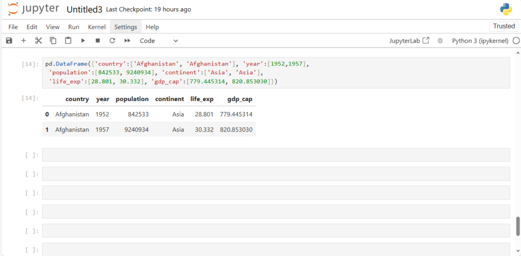
Handling Heterogeneous Data: Unlike NumPy, which primarily works with a single datatype (usually numeric), Pandas can handle heterogeneous data, meaning it can work with both numeric and string data in a dataset simultaneously. For example, you can store a combination of numeric data (like population) and string data (like place names) in a Pandas DataFrame.
Ease of Use: Pandas provides an intuitive syntax and powerful data structures (like Series and DataFrame) to make data manipulation easier. This is especially useful when dealing with complex datasets.

How is Pandas Different from NumPy?

While both NumPy and Pandas are excellent libraries for data manipulation, they are different in several ways:

NumPy: Works primarily with homogeneous data, meaning that all elements in an array are of the same type (e.g., all numbers).
Pandas: Provides more flexibility by supporting heterogeneous data types. You can work with numbers, strings, and other types of data in a single DataFrame.

Reading Dataset in Pandas

One of the most important features of Pandas is its ability to read data from different file formats like CSV, Excel, and SQL databases. Here’s how you can read a dataset from a CSV file:

df = pd.read_csv(r"C:\Users\welcome\Downloads\dataset1.csv")

After loading the dataset into a DataFrame (stored in the variable df), you can perform a wide range of operations like filtering, sorting, and analyzing the data.

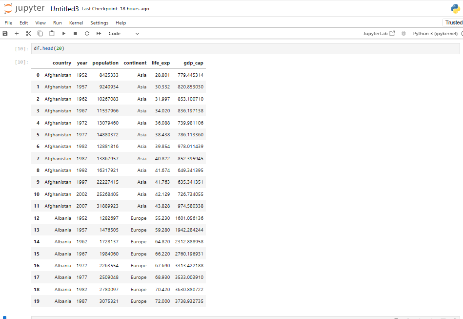
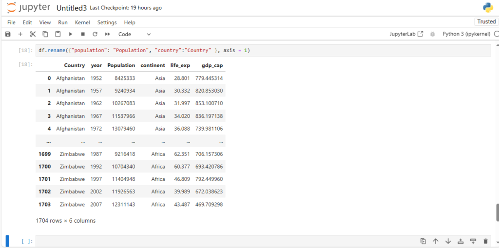
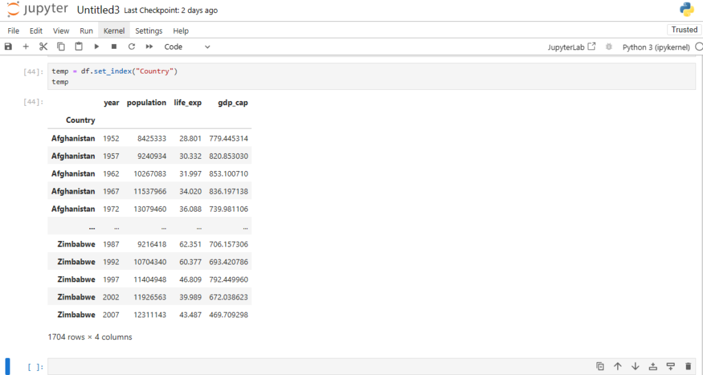
Exploring the Dataset

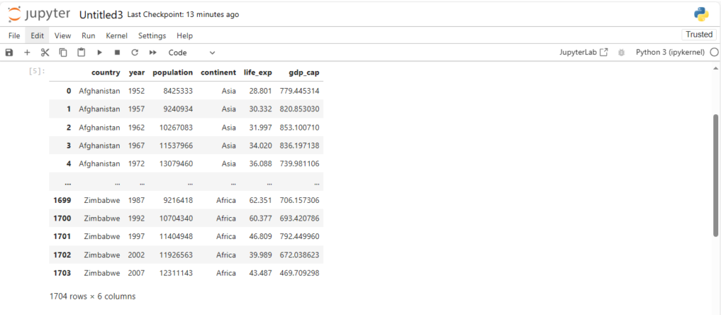
Once the dataset is loaded, you can simply print it using the command:

df

This will display the contents of the DataFrame. Pandas automatically handles the data types, formats, and data structure, making it much easier to explore and manipulate the data.

Exploring the Power of Pandas: A Comparison with NumPy

Importing Pandas

After installing Pandas, you can import it and start using it in your Python code. The common alias used for Pandas is pd. You can also import NumPy alongside Pandas for numerical operations, as shown below:

import pandas as pd
import numpy as np

Why Use Pandas?

Pandas is a Python library built for data analysis. Unlike NumPy, which only handles one data type at a time (like integers or floats), Pandas allows you to work with datasets that contain different types of data (such as integers, strings, and floats). This makes it a more versatile tool for real-world data analysis.

How is Pandas Different from NumPy?

While NumPy is excellent for mathematical computations and working with numerical data, it has a major limitation when it comes to handling heterogeneous data types. Most real-world datasets contain multiple data types. For example:

Names of cities are strings
Population is represented by integers

This makes NumPy less suited for such data. On the other hand, Pandas is designed to handle such mixed data efficiently, enabling you to perform operations on datasets with multiple data types seamlessly.

Pandas and Mixed Data Types

For instance, in a dataset about cities, you might have columns like:

City Name: A string (e.g., “New York”)
Population: An integer (e.g., 8,000,000)
Area: A float (e.g., 789.4 km²)

Pandas can handle such datasets with ease, unlike NumPy, which requires all data to be of the same type. Pandas offers the flexibility to work with structured, heterogeneous data.

Working with DataFrames in Pandas

Pandas provides the DataFrame object, which is similar to a table in a database or an Excel spreadsheet. DataFrames allow you to store, manipulate, and analyze data in a very flexible way. You can easily filter, group, and manipulate large datasets using simple commands in Pandas.

For example, you can read a CSV file into a Pandas DataFrame using the following code:

df = pd.read_csv('path/to/your/dataset.csv')
df.head()

Reading dataset in Pandas

df= pd.read_csv(r"C:\Users\welcome\Downloads\dataset1.csv")

Now how should we read this dataset?
Pandas makes it very easy to work with these kinds of files

df

Dataframe and Series

What can we observe from the above dataset ?
We can see that it has:

6 columns
1704 rows

what do you think is the datatype of df ?

type(df)

pandas.core.frame.DataFrame

Its a pandas DataFrame

What is a pandas DataFrame ?

It is a table-like representation of data in Pandas => Structured Data
Structured Data here can be thought of as tabular data in a proper order
Considered as counterpart of 2D-Matrix in Numpy

Now how can we access a column, say country of the dataframe?

df["country"]

Now what is the data-type of a column?

type(df["country"]) 

pandas.core.series.Series

Its a pandas Series

What is a pandas Series ?

Series in Pandas is what a Vector is in Numpy

What exactly does that mean?

It means a Series is a single column of data
Multiple Series stack together to form a DataFrame

Now we have understood what Series and DataFrames are

What if a dataset has 100 rows … Or 100 columns ?

How can we find the datatype, name, total entries in each column ?

df.info()

Now what if we want to see the first few rows in the dataset ?

df.head()

We can also pass in number of rows we want to see in head()

df.head(20)

Similarly what if we want to see the last 20 rows ?

df.tail(20) #Similar to head

How can we find the shape of the dataframe?

df.shape
(1704, 6)

Similar to Numpy, it gives No. of Rows and Columns — Dimensions
Now we know how to do some basic operations on dataframes

But what if we aren’t loading a dataset, but want to create our own.
Let’s take a subset of the original dataset

df.head(3) # We take the first 3 rows to create our dataframe

How can we create a DataFrame from scratch?

Approach 1: Row-oriented

It takes 2 arguments – Because DataFrame is 2-dimensional
A list of rows
Each row is packed in a list []
All rows are packed in an outside list [[]] – To pass a list of rows
A list of column names/labels

pd.DataFrame([['Afghanistan',1952, 8425333, 'Asia', 28.801, 779.445314 ],
['Afghanistan',1957, 9240934, 'Asia', 30.332, 820.853030 ],
['Afghanistan',1962, 102267083, 'Asia', 31.997, 853.100710 ]],
columns=['country','year','population','continent','life_exp','gdp_cap'])

Approach 2: Column-oriented

pd.DataFrame({'country':['Afghanistan', 'Afghanistan'], 'year':[1952,1957],
'population':[842533, 9240934], 'continent':['Asia', 'Asia'],
'life_exp':[28.801, 30.332], 'gdp_cap':[779.445314, 820.853030]})

We pass the data as a dictionary

Key is the Column Name/Label
Value is the list of values column-wise
We now have a basic idea about the dataset and creating rows and columns
What kind of other operations can we perform on the dataframe?
Thinking from database perspective:
Adding data
Removing data
Updating/Modifying data
and so on

How can we get the names of all these cols ?

We can do it in two ways:
1. df.columns
2. df.keys

df.columns # using attribute `columns` of dataframe

Index(['country', 'year', 'population', 'continent', 'life_exp', 'gdp_cap'], dtype='obje
ct')

df.keys() # using method keys() of dataframe

Index(['country', 'year', 'population', 'continent', 'life_exp', 'gdp_cap'], dtype='obje
ct')

Note:

Here, Index is a type of pandas class used to store the address of the series/dataframe
It is an Immutable sequence used for indexing and alignment.

df['country'].head() # Gives values in Top 5 rows pertaining to the key

But what is so “special” about this dictionary?

It can take multiple keys

df[['country', 'life_exp']].head()

And what if we pass a single column name?

df[['country']].head()

Note:

Notice how this output type is different from our earlier output using df[‘country’]
==> [‘country’] gives series while [[‘country’]] gives dataframe
Now that we know how to access columns, lets answer some questions

Now what if you also want to check the count of each country in the dataframe?

df['country'].value_counts()

Note:
value_counts() shows the output in decreasing order of frequency

What if we want to change the name of a column ?

We can rename the column by:

passing the dictionary with old_name:new_name pair
specifying axis=1

df.rename({"population": "Population", "country":"Country" }, axis = 1)

Alternatively, we can also rename the column without using axis

by using the column parameter

df.rename(columns={"country":"Country"})

We can set it inplace by setting the inplace argument = True

df.rename({"country": "Country"}, axis = 1, inplace = True)
df

Note:

.rename has default value of axis=0
If two columns have the same name, then df[‘column’] will display both columns

Now lets try another way of accessing column vals

df.Country

How can we delete cols in pandas dataframe ?

df.drop('continent', axis=1)

The drop function takes two parameters:

The column name
The axis

By default the value of axis is 0

An alternative to the above approach is using the “columns” parameter as we did in rename

df.drop(columns=['continent'])

As you can see, column contintent is dropped

Has the column permanently been deleted?

 df.head()

NO, the column continent is still there

Do you see what’s happening here?

We only got a view of dataframe with column continent dropped

How can we permanently drop the column?

We can either re-assign it

df = df.drop(‘continent’, axis=1)

We can set parameter inplace=True

By default, inplace=False

df.drop('continent', axis=1, inplace=True)

df.head() #we print the head to check

Now we can see the column continent is permanently dropped

Now similarly, what if we want to create a new column?

We can either

use values from existing columns

create our own values

How to create a column using values from an existing column?


df["year+7"] = df["year"] + 7
df.head()

As we see, a new column year+7 is created from the column year

We can also use values from two columns to form a new column

Which two columns can we use to create a new column gdp ?

df['gdp']=df['gdp_cap'] * df['population']
df.head()

As you can see

An additional column has been created
Values in this column are product of respective values in gdp_cap and population

How can we create a new column from our own values?

We can create a list

We can create a Pandas Series from a list/numpy array for our new column


df["Own"] = [i for i in range(1704)] # count of these values should be correct
df

Now that we know how to create new cols lets see some basic ops on rows

Before that lets drop the newly created cols

df.drop(columns=["Own",'gdp', 'year+7'], axis = 1, inplace = True)
df

Working with Rows

Notice the indexes in bold against each row

Lets see how can we access these indexes

df.index.values

array([ 0, 1, 2, ..., 1701, 1702, 1703], dtype=int64)

Can we change row labels (like we did for columns)?

What if we want to start indexing from 1 (instead of 0)?


df.index = list(range(1, df.shape[0]+1)) # create a list of indexes of same length
df

As you can see the indexing is now starting from 1 instead of 0.

Explicit and Implicit Indices

What are these row labels/indices exactly ?

They can be called identifiers of a particular row
Specifically known as explicit indices

The python style indices are known as implicit indices

How can we access explicit index of a particular row?

Using df.index[]
Takes impicit index of row to give its explicit index

 df.index[1] #Implicit index 1 gave explicit index 2 

2

But why not use just implicit indexing ?

Explicit indices can be changed to any value of any datatype

Eg: Explicit Index of 1st row can be changed to First
Or, something like a floating point value, say 1.0

df.index = np.arange(1, df.shape[0]+1, dtype='float')
df

As we can see, the indices are floating point values now

Now to understand string indices, let’s take a small subset of our original dataframe

sample = df.head()
sample

Now what if we want to use string indices?

sample.index = ['a', 'b', 'c', 'd', 'e']
sample

This shows us we can use almost anything as our explicit index

Now let’s reset our indices back to integers

df.index = np.arange(1, df.shape[0]+1, dtype='int')

What if we want to access any particular row (say first row)?

Let’s first see for one column

Later, we can generalise the same for the entire dataframe

ser = df["Country"]
ser.head(20)

We can simply use its indices much like we do in a numpy array

So, how will be then access the thirteenth element (or say thirteenth row)?

ser[12] 

'Afghanistan'

And what about accessing a subset of rows (say 6th:15th) ?

ser[5:15]

This is known as slicing

Notice something different though?

Indexing in Series used explicit indices
Slicing however used implicit indices

How can we access a slice of rows in the dataframe?

df[5:15]

Woah, so the slicing works
===> Indexing in dataframe looks only for explicit indices \ ===> Slicing, however, checked for implicit
indices
This can be a cause for confusion
To avoid this pandas provides special indexers, loc and iloc
We will look at these in a bit Lets look at them one by one

loc and iloc

1. loc

Allows indexing and slicing that always references the explicit index

df.loc[1]

Country                       Afghanistan
year                                 1952
population                        8425333
life_ex                            28.801
gdp_cap                        779.445314
Name:    1, dtype: object

df.loc[1:3]

Did you notice something strange here?

The range is inclusive of end point for loc
Row with Label 3 is included in the result

2. iloc

Allows indexing and slicing that always references the implicit Python-style index

df.iloc[1]

Country        Afghanistan
year                  1957
population         9240934
life_exp            30.332
gdp_cap          820.85303
Name: 2, dtype: object

Now will iloc also consider the range inclusive?

df.iloc[0:2]

iloc works with implicit Python-style indices

It is important to know about these conceptual differences

Not just b/w loc and iloc , but in general while working in DS and ML

Which one should we use ?

Generally explicit indexing is considered to be better than implicit
But it is recommended to always use both loc and iloc to avoid any confusions

What if we want to access multiple non-consecutive rows at same time ?

For eg: rows 1, 10, 100

df.iloc[[1, 10, 100]]

As we see, We can just pack the indices in [] and pass it in loc or iloc

What about negative index?

Which would work between iloc and loc ?

 df.iloc[-1]
# Works and gives last row in dataframe

Country         Zimbabwe
year                2007
population      12311143
life_exp          43.487
gdp_cap       469.709298
Name: 1704, dtype: object

df.loc[-1]
# Does NOT work

So, why did iloc[-1] worked, but loc[-1] didn’t?

Because iloc works with positional indices, while loc with assigned labels
[-1] here points to the row at last position in iloc

Can we use one of the columns as row index?

temp = df.set_index("Country")
temp

Now what would the row corresponding to index Afghanistan give?

temp.loc['Afghanistan']

As you can see we got the rows all having index Afghanistan

Now how can we reset our indices back to integers?

df.reset_index()

Notice it’s creating a new column index

How can we reset our index without creating this new column?

df.reset_index(drop=True) # By using drop=True we can prevent creation of a new column

Great, now let’s do this in place

df.reset_index(drop=True, inplace=True)

Now how can we add a row to our dataframe?

There are multiple ways to do this:

append()
loc/iloc

How can we do add a row using the append() method?

new_row = {'Country': 'India', 'year': 2000,'life_exp':37.08,'population':13500000,'gdp_
df.append(new_row)

Why are we getting an error here?

Its’ saying the ignore_index() parameter needs to be set to True


new_row = {'Country': 'India', 'year': 2000,'life_exp':37.08,'population':13500000,'gdp_
df = df.append(new_row, ignore_index=True)
df

What you can infer from last two duplicate rows ?

Dataframe allow us to feed duplicate rows in the data

Now, can we also use iloc?

Adding a row at a specific index position will replace the existing row at that position.


df.iloc[len(df.index)-1] = ['India', 2000,13500000,37.08,900.23]
df

Now what if we want to delete a row ?

Use df.drop()

If you remember we specified axis=1 for columns
We can modify this for rows

We can use axis=0 for rows

Does drop() method uses positional indices or labels?

What do you think by looking at code for deleting column?

We had to specify column title
So drop() uses labels, NOT positional indices


# Let's drop row with label 3
df = df.drop(3, axis=0)
df

Now we see that row with label 3 is deleted

We now have rows with labels 0, 1, 2, 4, 5, …

Now df.loc[4] and df.iloc[4] will give different rows

df.loc[4] # The 4th row is printed

Country        Afghanistan
year                 1972
population       13079460
life_exp           36.088
gdp_cap       739.981106
Name: 4, dtype: object

df.iloc[4] # The 5th row is printed

Country        Afghanistan
year                  1977
population         14880372
life_exp             38.438
gdp_cap            786.11336
Name: 5, dtype: object

And hww can we drop multiple rows?

df.drop([1, 2, 4], axis=0) # drops rows with labels 1, 2, 4

Let’s reset our indices now

df.reset_index(drop=True,inplace=True)

Now if you remember, the last two rows were duplicates.

How can we deal with these duplicate rows?

Let’s create some more duplicate rows to understand this


df.loc[len(df.index)] = ['India',2000,13500000,37.08,900.23]
df.loc[len(df.index)] = ['Sri Lanka',2022 ,130000000,80.00,500.00]
df.loc[len(df.index)] = ['Sri Lanka',2022 ,130000000,80.00,500.00]
df.loc[len(df.index)] = ['India',2000 ,13500000,80.00,900.23]
df

Now how can we check for duplicate rows?

Use duplicated() method on the DataFrame

df.duplicated()

0         False
1          False
2         False
3         False
4         False
... 
1703       False
1704       True
1705       False
1706       True
1707        False
Length: 1708, dtype: bool

It outputs True if an entire row is identical to a previous row.

However, it is not practical to see a list of True and False

We can Pandas loc data selector to extract those duplicate rows


# Extract duplicate rows
df.loc[df.duplicated()]

Working with Rows and Columns together

How can we slice the dataframe into, say, first 4 rows and first 3 columns?

We can use iloc

df.iloc[1:5, 1:4]

Pass in 2 different ranges for slicing – one for row and one for column just like Numpy
Recall, iloc doesn’t include the end index while slicing

We can mention ranges using column labels as well in loc

df.loc[1:5, 'year':'population']

How can we get specific rows and columns?

df.iloc[[0,10,100], [0,2,3]]

We pass in those specific indices packed in []

Can we do step slicing?

Yes, just like we did in Numpy

df.iloc[1:10:2]

Does step slicing work for loc too?

df.loc[1:10:2]

Pandas built-in operation

Let’s select the feature ‘life_exp‘

le = df['life_exp']
le

How can we find the mean of the col life_exp ?

 le.mean()
=> 59.499171358313774

What other operations can we do?

sum()
count()
min()
max()

… and so on

Note:
We can see more methods by pressing “tab” after le.

   le.sum()
=> 101624.58468

  le.count()
=>1708

What will happen we get if we divide sum() by count() ?

   le.sum() / le.count()
=> 59.499171358313816

It gives the mean of life expectancy

Sorting

If you notice, life_exp col is not sorted

How can we perform sorting in pandas ?

df.sort_values(['life_exp'])

Rows get sorted based on values in life_exp column

By default, values are sorted in ascending order

How can we sort the rows in descending order?

df.sort_values(['life_exp'], ascending=False)

Now the rows are sorted in descending

Can we do sorting on multiple columns?

df.sort_values(['year', 'life_exp'])

What exactly happened here?

Rows were first sorted based on ‘year‘
Then, rows with same values of ‘year’ were sorted based on ‘lifeExp‘

This way, we can do multi-level sorting of our data?

How can we have different sorting orders for different columns in multi-level sorting?

df.sort_values(['year', 'life_exp'], ascending=[False, True])

Just pack True and False for respective columns in a list []

Concatenating DataFrames

Let’s use a mini use-case of users and messages

users –> Stores the user details – IDs and Names of users

users = pd.DataFrame({"userid":[1, 2, 3], "name":["kiran", "alok", "vikas"]})
users

msgs –> Stores the messages users have sent – User IDs and messages

msgs = pd.DataFrame({"userid":[1, 1, 2, 4], "msg":['ok', "thik", "wow", "hmm"]})
msgs

Can we combine these 2 DataFrames to form a single DataFrame?

pd.concat([users, msgs])

How exactly did concat work?

By default, axis=0 (row-wise) for concatenation
userid , being same in both DataFrames, was combined into a single column

First values of users dataframe were placed, with values of column msg as NaN
Then values of msgs dataframe were placed, with values of column msg as NaN

The original indices of the rows were preserved

Now how can we make the indices unique for each row?

pd.concat([users, msgs], ignore_index = True)

How can we concatenate them horizontally?

pd.concat([users, msgs], axis=1)

As you can see here:

Both the dataframes are combined horizontally (column-wise)
It gives 2 columns with different positional (implicit) index, but same label

Merging Dataframes

So far we have only concatenated and not merged data

But what is the difference between concat and merge ?

concat

simply stacks multiple DataFrame together along an axis

merge

combines dataframes in a smart way based on values in shared columns

How can we know the name of the person who sent a particular message?

We need information from both the dataframes

So can we use pd.concat() for combining the dataframes ?

pd.concat([users, msgs], axis=1)

What are the problems with concat here?

concat simply combined/stacked the dataframe horizontally
If you notice, userid 3 for user dataframe is stacked against userid 2 for msg dataframe
This way of stacking doesn’t help us gain any insights

=> pd.concat() does not work according to the values in the columns

We need to merge the data

How can we join the dataframes ?

users.merge(msgs, on="userid")

Notice that users has a userid = 3 but msgs does not

When we merge these dataframes the userid = 3 is not included
Similarly, userid = 4 is not present in users , and thus not included
Only the userid common in both dataframes is shown

What type of join is this?

Inner Join

Remember joins from SQL?

The on parameter specifies the key , similar to primary key in SQL

Now what join we want to use to get info of all the users and all the messages?

 users.merge(msgs, on = "userid", how="outer")

Note:

All missing values are replaced with NaN

And what if we want the info of all the users in the dataframe?

users.merge(msgs, on = "userid",how="left")

what if we want all the messages and info only for the users who sent a message?

users.merge(msgs, on = "userid", how="right")

Note,

NaN in name can be thought of as an anonymous message

But sometimes the column names might be different even if they contain the same data

Let’s rename our users column userid to id

users.rename(columns = {"userid": "id"}, inplace = True)
users

how can we merge the 2 dataframes when the key has a different name ?

 users.merge(msgs, left_on="id", right_on="userid")

Here,

left_on : Specifies the key of the 1st dataframe (users here)
right_on : Specifies the key of the 2nd dataframe (msgs here)

Choose the Right Program for Your Career in Data Analytics

Unlock Your Future with Our Data Analytics Courses

Interested in building a career in the dynamic world of data analytics? Our data analytics courses at Vista Academy are crafted to provide you with the essential skills and expertise to thrive in this rapidly expanding field. Through a combination of theoretical knowledge and hands-on experience, you’ll be equipped to excel in the ever-evolving world of data.

Why Choose Our Data Analytics Program?

Experienced Instructors: Learn from seasoned professionals with extensive industry experience.
Hands-On Projects: Apply your knowledge through real-world simulations and case studies that reflect industry practices.
Practical Learning Environment: Gain practical insights and develop skills that are directly applicable in the workforce.
Data-Driven Decision-Making: Master how to analyze data and craft insightful reports that inform business strategy.

Real-World Experience & Skill Development

Our curriculum emphasizes real-world applications, ensuring that you not only gain theoretical knowledge but also acquire the practical skills necessary to excel in data analytics. You’ll be able to create data-driven reports and make decisions that can drive business success.

Enroll Now & Start Your Data Analytics Journey

Data Analytics and Data Science course in Dehradun Uttarakhand

Data Analytics and Data Science course in Dehradun Uttarakhand