Table of Contents
ToggleDiscover how Linear Regression works in Data Analytics with a complete step-by-step guide. Learn theory and practice with Python, Excel, and Power BI through real-world examples, business use cases, and hands-on tutorials.
Data is the new oil — but raw data alone has little value. It’s the insights hidden within that drive growth, strategy, and innovation. This is where Data Analytics steps in, and at the very foundation of predictive analytics lies Linear Regression.
Linear Regression is more than just a math equation — it’s a way to predict the future using past data. Whether it’s estimating house prices, forecasting product sales, or analyzing stock market trends, this technique is one of the simplest yet most powerful tools in analytics.
In simple words, Linear Regression helps you find the relationship between a set of factors and an outcome. It predicts a dependent variable (Y) using one or more independent variables (X).
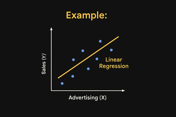
Imagine you are a marketing manager. You want to know how much Sales (Y) will increase if you spend more on Advertising (X).
Linear Regression helps you draw that line of best fit, showing how Sales are linked with Ad Spend.
Forecasting seasonal product demand & sales growth.
Estimating student performance from study hours & attendance.
Predicting house prices using size, location & facilities.
Analyzing effect of exercise & diet on patient recovery.
Predicting stock returns & investment risks.
Mastering Linear Regression in Data Analytics is your first step towards becoming a skilled Data Analyst or Data Scientist. In the upcoming sections, we’ll explore its types, formulas, and hands-on implementation in Python, Excel, and Power BI.
Linear Regression comes in different forms based on the number of predictor variables—let’s explore the two most common types: Simple and Multiple Linear Regression.
Applicable when analyzing the relationship between one independent variable (X) and one dependent variable (Y). The model looks like this:
Y = β₀ + β₁X + ε – β₀: Intercept (Y-value when X = 0) – β₁: Slope (effect of X on Y) – ε: Error term
Predicting Sales (Y) based on Advertising Spend (X). As ad spend increases, sales typically follow a linear trend.
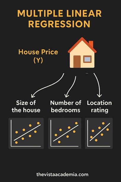
Used when predicting Y using **two or more independent variables** (X₁, X₂, …). The model becomes:
Y = β₀ + β₁X₁ + β₂X₂ + … + βₙXₙ + ε
Predicting House Price (Y) using factors like: • House Size (X₁) • Number of Bedrooms (X₂) • Location Rating (X₃) Each contributes uniquely to the final price estimate.
• Use **Simple Linear Regression** when examining a single influence on the outcome.
• Choose **Multiple Linear Regression** when multiple factors drive the result.
Next up: we’ll dive into the **key assumptions of Linear Regression**—so your predictions stay reliable and valid.
To get reliable and accurate results from a Linear Regression model, certain statistical assumptions must be satisfied. Ignoring these can lead to misleading predictions and incorrect conclusions.
The relationship between the independent variable(s) (X) and the dependent variable (Y) should be linear. Example: As ad spend increases, sales increase in a straight-line fashion.
Residuals (errors) should be independent of each other. This means one prediction’s error should not influence another’s.
The variance of residuals should remain constant across all levels of X. If residuals spread out unevenly, predictions may be biased.
The residuals should follow a normal distribution. This assumption is especially important for hypothesis testing and confidence intervals.
In Multiple Linear Regression, independent variables should not be highly correlated with each other. Example: If House Size and Number of Rooms are almost identical, it creates redundancy.
(Illustration: Core assumptions of Linear Regression)
Violating these assumptions may still allow a model to run, but the predictions could be unreliable. Understanding them ensures your Data Analytics workflow remains accurate, interpretable, and trusted.
The power of Linear Regression lies in its mathematical formula, which helps us draw the best-fit line between variables and make predictions.
Y = β₀ + β₁X + ε
Where:
• Y = Dependent variable (outcome to predict)
• X = Independent variable (predictor)
• β₀ = Intercept (value of Y when X = 0)
• β₁ = Slope (how much Y changes with 1 unit change in X)
• ε = Error term (difference between predicted and actual values)
Y = β₀ + β₁X₁ + β₂X₂ + β₃X₃ + … + βₙXₙ + ε
Here, multiple predictors (X₁, X₂, X₃ … Xₙ) contribute to predicting the same outcome (Y). Example: Predicting house prices using size, location, and number of rooms.
Suppose the regression model is:
Sales = 50 + 2 × (Ad Spend)
• Intercept (50): Even if ad spend is 0, expected sales = 50 units.
• Slope (2): For every ₹1 increase in ad spend, sales increase by 2 units.
👉 If Ad Spend = ₹100, then: Sales = 50 + 2 × 100 = 250 units.
(Interactive Chart: Regression Line for Sales vs Ad Spend)
Understanding the formula helps analysts interpret regression results, explain the impact of predictors,
and make data-driven business decisions.
Next, we’ll explore a step-by-step example of Linear Regression using a simple dataset.
Let’s walk through a practical example of Linear Regression in Data Analytics using a small dataset. We’ll predict Sales based on Advertising Spend.
Ad Spend (₹) | Sales (Units) |
---|---|
50 | 150 |
100 | 250 |
150 | 350 |
200 | 450 |
250 | 550 |
• Independent Variable (X) = Advertising Spend (₹) • Dependent Variable (Y) = Sales (Units)
If we plot Ad Spend on the X-axis and Sales on the Y-axis, the data points show a clear upward trend.
The best-fit line is calculated using the regression formula:
Sales = 50 + 2 × (Ad Spend)
• Intercept = 50
• Slope = 2 (for every ₹1 increase in ad spend, sales rise by 2 units)
If Ad Spend = ₹300, then: Sales = 50 + 2 × 300 = 650 units.
(Interactive Visualization: Example of Linear Regression with Sales vs Ad Spend)
Python is one of the most powerful tools for Data Analytics. With libraries like pandas, NumPy, matplotlib, and scikit-learn, running Linear Regression becomes simple and efficient.
import pandas as pd from sklearn.linear_model import LinearRegression
We import pandas for handling data and LinearRegression from scikit-learn to build our model.
data = { 'Ad_Spend': [50, 100, 150, 200, 250], 'Sales': [150, 250, 350, 450, 550] } df = pd.DataFrame(data)
We use the same dataset (Ad Spend vs Sales) for consistency.
X = df[['Ad_Spend']] y = df['Sales'] model = LinearRegression() model.fit(X, y) print("Intercept:", model.intercept_) print("Slope:", model.coef_)
Here, the model calculates: • Intercept = 50 • Slope = 2
predicted_sales = model.predict([[300]]) print("Predicted Sales for ₹300 ad spend:", predicted_sales[0])
👉 For ₹300 ad spend, predicted sales = 650 units.
• The model learns the relationship between Ad Spend and Sales. • It uses the formula Sales = 50 + 2 × (Ad Spend). • When new data is provided, the model can predict future sales.
Excel is widely used in business and corporate settings. It provides simple yet effective ways to perform Linear Regression without coding.
✅ This will show the regression line, equation (e.g., Sales = 50 + 2 × Ad Spend) and R² (goodness of fit).
✅ Excel generates a detailed regression output with coefficients, R² value, and significance levels.
Regression Equation: Sales = 50 + 2 × Ad Spend | R² = 1.00
Power BI is not just for dashboards — it can also perform Linear Regression. Let’s explore how to implement regression models step by step in Power BI.
• Load your dataset (Ad Spend vs Sales) into Power BI. • Use a Scatter Chart visualization. • Enable the Analytics → Trendline option. • Power BI automatically fits a regression line.
You can also calculate regression line values manually with DAX. Example formula for Sales Prediction:
Predicted Sales = 50 + 2 * SUM('Data'[Ad_Spend])
Here, 50 is the intercept and 2 is the slope.
Power BI allows you to run Python scripts directly inside visuals. By importing scikit-learn, you can run the same Python regression model we used earlier.
Regression Equation: Sales = 50 + 2 × Ad Spend | R² = 1.00
From forecasting sales to optimizing marketing budgets, Linear Regression powers everyday business decisions. Below are real-world applications you can adapt to your projects.
Build a mini project: pick any two predictors and a business KPI, run a regression in Python, replicate visuals in Excel/Power BI, and explain the coefficients in plain English.
You’ve learned how Linear Regression works—from the formula and assumptions to hands-on implementation in Python, Excel, and Power BI. It’s simple, interpretable, and incredibly useful for everyday analytics like sales forecasting, budget planning, and marketing ROI.
Predict a numeric outcome (Y) from one or more inputs (X) using a best-fit line.
Simple: 1 predictor. Multiple: 2+ predictors (X₁…Xₙ).
Linearity, independent errors, homoscedasticity, normal residuals, low multicollinearity.
Excel for quick checks, Power BI for dashboards, Python for production/scale.
Pick a business KPI (Sales, Revenue, Leads). Choose 2–3 drivers (Ad Spend, Price, Season). Build a regression in Python/Excel/Power BI, visualize it, and explain each coefficient in plain English.
Join Vista Academy’s Free Sunday Demo ClassIt’s a method to predict a numeric outcome by drawing a straight line that best fits the relationship between inputs (X) and output (Y).
Simple uses one predictor (X). Multiple uses two or more predictors (X₁…Xₙ) to explain Y better.
R² shows how much of the variance in Y is explained by the model (0–1). Higher is better, but always check assumptions and overfitting.
Python: Use LinearRegression
from scikit-learn.
Excel: Scatter plot → Trendline, or Data Analysis → Regression (ToolPak).
Power BI: Scatter chart with Trendline, DAX measures, or Python scripts.
Avoid when relationships are clearly non-linear, there are many outliers, or predictors are highly collinear. Consider tree-based models or regularization.
Yes—if the relationship stays stable and assumptions hold. For time series, prefer methods that respect time order (e.g., trend/seasonality models).
Excel: Quick checks and presentations.
Power BI: Interactive dashboards with trendlines and DAX.
Python: Best for automation, scale, MLOps, and deeper evaluation.
Practice Linear Regression with these datasets, notebooks, and templates across Python, Excel, and Power BI.
Use the Google Sheet as a source, or download as CSV for Excel / connect via Web in Power BI.
⬇ Download CSVPower BI tip: Get data → Web → use the CSV link above.
Train, predict, and visualize Linear Regression in a Jupyter/Anaconda environment.
⬇ Open Python NotebookConnect Power BI directly to the Google Sheet (or the CSV link) and add a Trendline to your Scatter chart.
🔗 Open Data Source (Sheet)Or use CSV via: Get data → Web → paste the CSV link above.
Mastering Linear Regression is just the first step in your Data Analytics & Machine Learning journey. Explore more advanced models and practical business use cases with Vista Academy.
Learn how analytics drives decision-making in finance, HR, marketing, and operations.
→ Explore Business AnalyticsGo beyond regression! Learn Logistic Regression, Decision Trees, and Neural Networks.
→ Start Machine LearningLearn Python, Excel, SQL, and Power BI to become a job-ready Data Analyst.
→ Learn Data AnalyticsKeep practicing with real datasets. The more you experiment with Python, Excel, and Power BI, the more confident you’ll become in solving real business problems using Data Analytics.
Answer the questions and click Submit to see your score, correct answers, and explanations. You can retake the quiz anytime.
Vista Academy • Linear Regression MCQ • Interactive