📈 Compound Interest Formula in Excel
Table of Contents
ToggleTo calculate compound interest in Excel, use this manual formula:
=P*(1 + R/N)^(N*T)- P = Principal
- R = Annual interest rate (in decimal, e.g., 8% = 0.08)
- N = Number of times interest is compounded per year (e.g., 12 for monthly)
- T = Number of years
📌 Example (Step-by-Step):
Suppose you invest ₹10,000 at an annual interest rate of 8%, compounded monthly, for 5 years.
Use this formula in Excel:
=10000*(1 + 0.08/12)^(12*5)Result: ₹14,898.46 (approximately)
This is the future value of your investment after 5 years with compound interest.
✅ Using Built-in Excel Function (FV):
You can also calculate compound interest using Excel’s built-in =FV() function.
=FV(8%/12, 12*5, 0, -10000)- Rate = 8%/12 (monthly interest)
- Nper = 12*5 (total months)
- Pmt = 0 (no additional monthly payment)
- PV = -10000 (negative because it’s an investment)
Output: ₹14,898.46
👉 This formula tells you how much your ₹10,000 investment will grow in 5 years with monthly compounding.
PMT: Financial Function in Excel
PMT PERIODICAL PAYMENT REQUIRED
In excel, PMT denotes the periodical payment required to pay off for a particular period with a constant interest rate. Let’s have a look at how to calculate it in excel –
PMT – Financial Functions in Excel
PMT = (Rate, Nper, PV, [FV], [Type])
Rate = It is the interest rate/period
Nper = Number of periods
PV = Present Value
[FV] = An optional argument which is about the future value of a loan (if we mentioned nothing, FV is considered as “0”)
[Type] = When the payment is made (if we mentioned nothing, it’s assumed that we have made the payment at the end of the period)
PMT Example
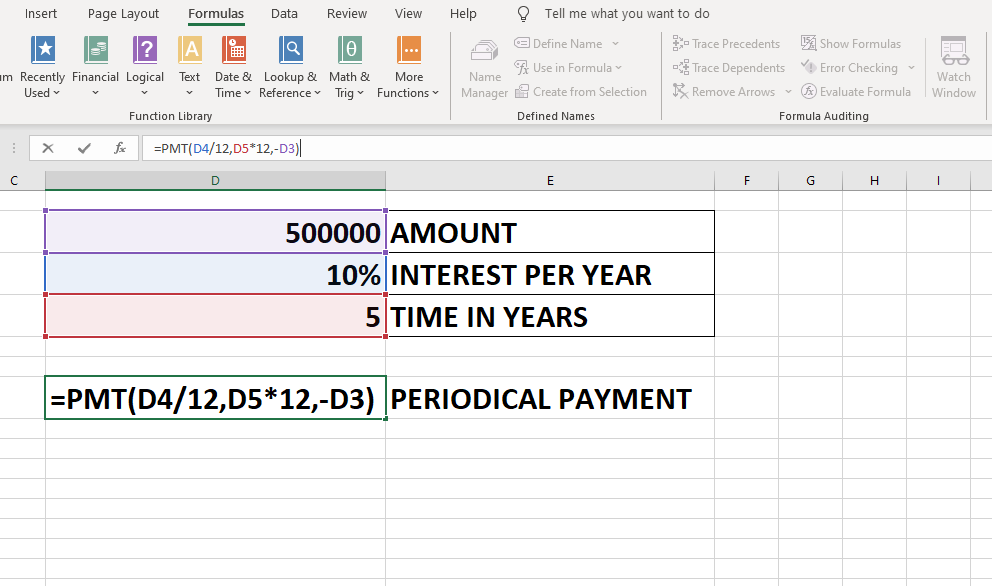
The Rs. 500000 needs to be paid in full in 5 years. The interest rate is 10% p.a. and the payment needs to be done yearly. Find out the PMT.
Solution: In excel, we will calculate it in the following manner –
PMT – Financial Functions in Excel Example
= =PMT(D4/12,D5*12,-D3)
- In this rate is divided by 12 to know the rate per month
- Nper number is multiply by 12 to know the number of installment per month.
- put – in present value as the money need to be give .
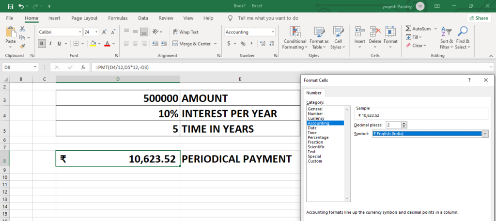
- Chang currency from $ to Rupee by home tab >number >accounting and change currency to Rupee
Change symbol of currency from dollar to rupee
IPMT Financial Function in Excel
IPMT function in excel
IPMT function in excel is used to calculate the interest to be paid on a loan where the interest and periodic payments are constant, this is an inbuilt function in excel and is also a type of financial function, this function calculates the portion of interest for the payment done for a period.
=IPMT (rate, per, nper, pv, [fv], [type])
Arguments
rate – The interest rate per period.
per – The payment period of interest.
nper – The total number of payment periods.
pv – The present value, or total value of all payments now.
fv – [optional] The cash balance desired after last payment is made. Defaults to 0.
type – [optional] When payments are due. 0 = end of period. 1 = beginning of period. Default is.
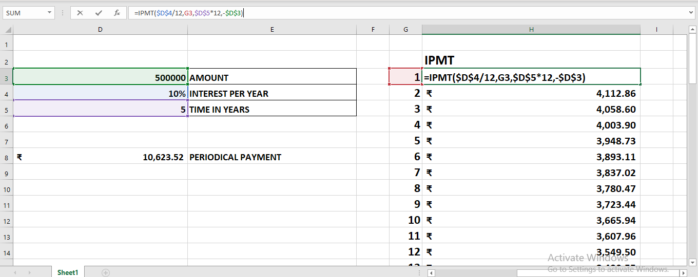
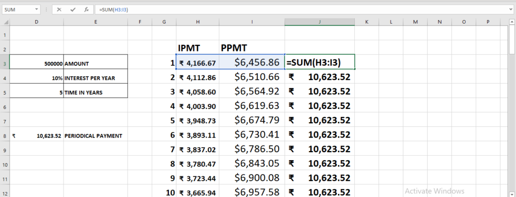
The Rs 50000 needs to be paid in full in 5 years. The interest rate is 10% p.a. and the payment needs to be done yearly.
In the example below per has been used to find out the period of payment which keeps on changing.
Drag number of payment from 1 to 60.as given below.
=IPMT($D$4/12,G6,$D$5*12,-$D$3)
PPMT function in excel
PPMT – Financial Functions in Excel
PPMT = (Rate, Per, Nper, PV, [FV], [Type])
Rate = It is the interest rate/period
Per = The period for which the principal is to be calculated
Nper = Number of periods
PV = Present Value
[FV] = An optional argument which is about the future value of a loan (if nothing is mentioned, FV is considered as “0”)
[Type] = When the payment is made (if nothing is mentioned, it’s assumed that the payment has been made at the end of the period)
PPMT Example
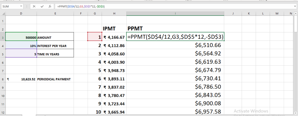
The Rs 50000 needs to be paid in full in 5 years. The interest rate is 10% p.a. and the payment needs to be done yearly.
Solution: In excel, we will calculate it in the following manner –
1st year,
PPMT – Financial Functions in Excel Example 1
=
 Interest Formula in Excel
Basic interest calculation:
=Principal * Rate * TimeExample: =A2*B2*C2 where D3 = Principal, D4= Rate, D5 = Time
FV function in Excel
FUTURE VALUE FORMULA
The Formula
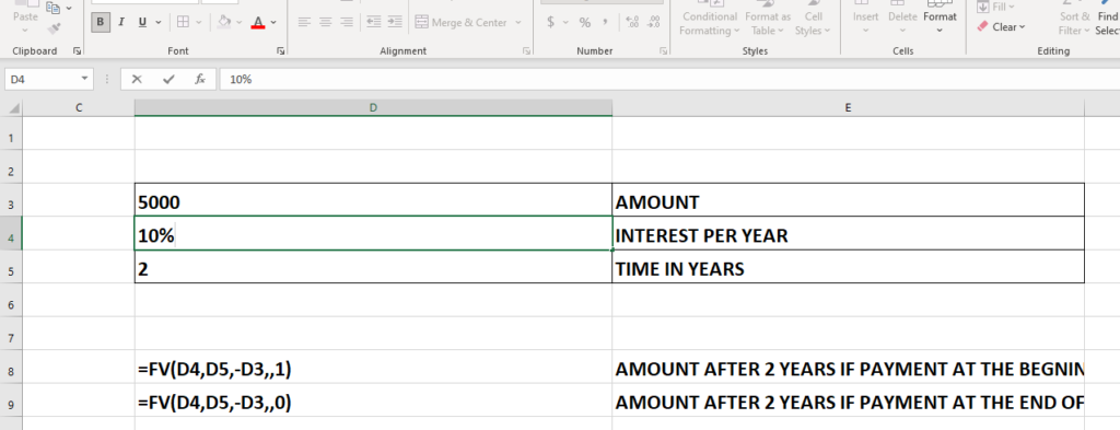
=FV(rate,nper,pmt,[pv],[type])
This function uses the following arguments:
- Rate (required argument)—This is the interest rate for each period.
- Nper (required argument)–The total number of payment periods.
- Pmt (optional argument)–This specifies the payment per period. If we omit this argument, we need to provide the PV argument.
- PV (optional argument) – This specifies the present value (PV) of the investment/loan. The PV argument, if omitted, defaults to zero. If we omit the argument, we need to provide the Pmt argument.
- Type (optional argument) – This defines whether payments are made at start or end of the year. The argument can either be 0 (it makes payment at the end of the period) or 1 (it makes the payment at the start of the period).
💸 FV (Future Value) Formula in Excel
Syntax: =FV(rate, nper, pmt, [pv], [type])
Example: =FV(6%/12, 12*5, -1000, -10000)
This returns the future value of an investment where:
- Rate = interest rate
- Nper = total periods
- Pmt = periodic payment
- PV = present value
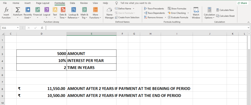
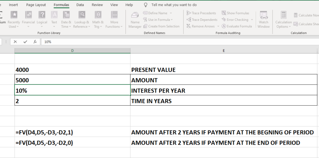
Suppose we have Rs 4000 at our bank account now we contribute 5000 yearly.
Case 1 at the beginning of the period.
Case 2 at the end of peroid.
Straight Line Depreciation (SLN) in Excel
The SLN function
uses the following arguments:
Cost (required argument) – This is the initial cost of the asset.
Salvage (required argument) – The value at the end of the depreciation (sometimes called the salvage value of the asset).
Life (required argument) – This is the number of periods over which the asset is depreciated (sometimes called the useful life of the asset).
What is salvage value ?
The salvage value of an asset is based on what a company expects to receive in exchange for selling or parting out the asset at the end of its useful life
Notes
Straight-line depreciation is the simplest way of calculating the depreciation of a fixed asset.
The formula used in calculating straight-line depreciation is:
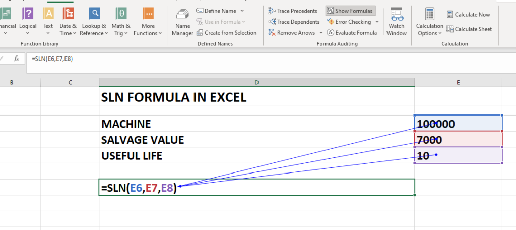
SLN = cost – salvage / life
Suppose A comapnay have a machine with value of machine is 100000 its salvage value Rs 7000 after 10 years.
DB Function in Excel
DB Function in Excel
The Excel DB function returns the depreciation of an asset for a specified period using the fixed-declining balance method. The calculation is based on initial asset cost, salvage value, the number of periods over which the asset is depreciated and, optionally, the number of months in the first year.in Excel..
The Excel DB function calculates the depreciation of an asset, using the Fixed Declining Balance Method, for each period of the asset’s lifetime.
The syntax of the function is:
DB( cost, salvage, life, period, [month] )
where the arguments are:
cost – The initial cost of the asset.
salvage – The value of the asset at the end of the depreciation.
life – The number of periods over which the asset is to be depreciated.
period – The period number for which we want to calculate the depreciation.
[month] –
An optional integer argument that specifies how many months of the year are used in the calculation of the first period of depreciation.
The number of months in the last period of depreciation is then calculated as 12 – [month].
If the [month] argument is omitted, it takes the default value of 12.
Example
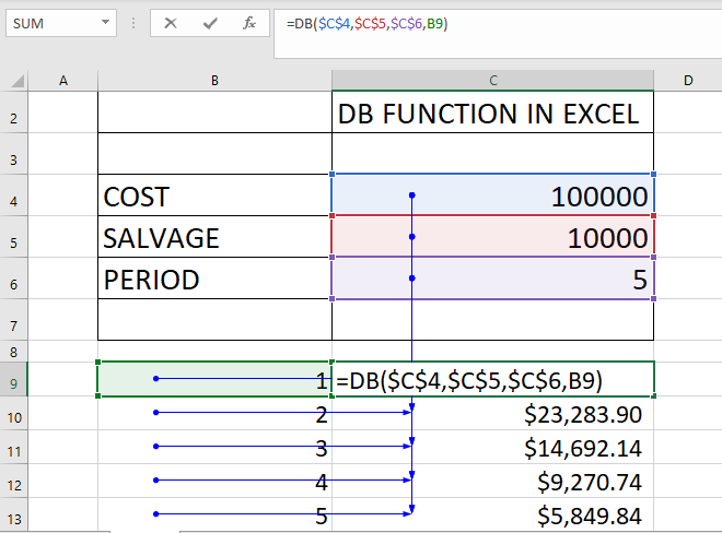
The DB function is used to find the yearly depreciation of an asset that costs Rs 100,000 at the start of year 1, and has a salvage value of Rs. 10,000 after 5 years.
Example 2
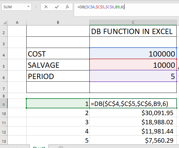
In the example below, the DB function is used with the same cost, salvage and life argument values as in Example 1 above. However, in the following example, the depreciation calculation starts 6 months into year 1.”
Variable Declining Balance in excel
Purpose
Depreciation – double-declining variable
Return value
Depreciation in given period
Syntax
=VDB (cost, salvage, life, start, end, [factor], [no_switch])
Arguments
cost
– Initial cost of asset.
salvage
Asset value at the end of the depreciation.
life –
Periods over which asset is depreciated.
start –
Start period.
end –
End period.
Factor
The rate at which the balance declines.
If factor is omitted, it is assumed to be 2 (the double-declining balance method).
Change factor if you do not want to use the doubledeclining balance method.
For a description of the double-declining balance method, refer DDB Function.
Optional
No_switch
A logical value specifying whether to switch to straight-line depreciation when depreciation is greater than the declining balance calculation.
If no_switch is TRUE, Excel does not switch to straight-line depreciation even when the depreciation is greater than the declining balance calculation.
If no_switch is FALSE or omitted, Excel switches to straight-line depreciation when depreciation is greater than the declining balance calculation.
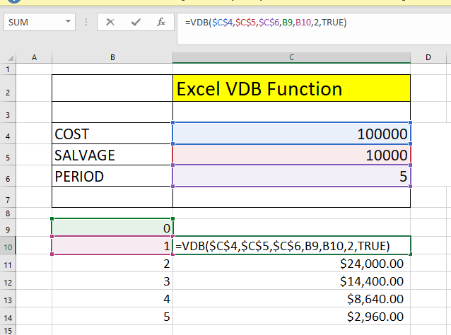
We wish to calculate the depreciation for an asset with an initial cost of Rs.500,000 and a salvage value of Rs.50,000 after 5 years.
We will calculate the depreciation for one day, one month, and one year. The formula used in calculating depreciation for a day is RS.
Net present value (NPV) in Excel
Net present value (NPV)
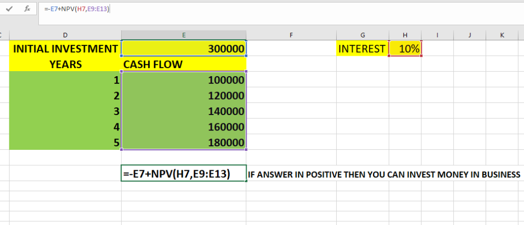
This is part of Capital budgeting in accounting.The Excel NPV function is a financial function that calculates the net present value (NPV) of an investment using a discount rate and a series of future cash flows.
Formula:
=NPV (rate, value1, [value2], …)
- rate – Discount rate over one period.
- value1 – First value(s) representing cash flows.
- value2 – [optional] Second value(s) representing cash flows.
A Company first put some money is beginning it is known as initial investment and later the company give some profit in coming year . The rate here describe is that money which business put in FD or other investment, what interest that money will pay. if not invested in business.
Now we have to calculate NPV to know whether to invest money in business or not that depends upon the answer of NPV
IRR FORMULA IN EXCEL
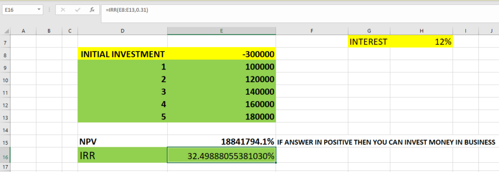
The Excel IRR function is a financial function that returns the internal rate of return (IRR) for a series of cash flows that occur at regular intervals.
=IRR (values, [guess])
values – Array or reference to cells that contain values.
guess – [optional] An estimate for expected IRR. Default is .1 (10%).
XIRR FUNCTION IN EXCEL
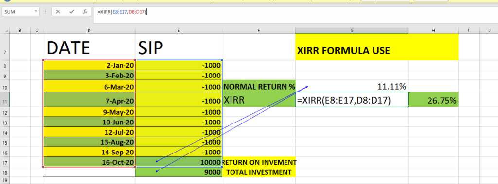
It will calculate the Internal Rate of Return (IRR) for a series of cash flows that may not be periodic. It does this by assigning specific dates to each individual cash flow. The main benefit of using the XIRR Excel function is that such unevenly timed cash flows can be accurately modeled,
The formula uses the following arguments:
- Values (required argument) – This is the array of values that represent the series of cash flows. Instead of an array, it can be a reference to a range of cells containing values.
- Dates (required argument) – This is a series of dates that correspond to the given values. Subsequent dates should be later than the first date, as the first date is the start date and subsequent dates are future dates of outgoing payments or income.
- [guess] (optional argument) – This is an initial guess – or estimate – of what the IRR will be. If omitted, Excel takes the default value of 10%.
In example below we are calculaing XIRR on SIP of 1000 each month for 9 month and in 10 month we find the return on investment one way is to find it normal rate of returns which is
NORMAL RATE OF RETURN =RETURN ON INVESTMENT / TOTAL INVESTMENT -1
Whereas XIRR calculate more accurate return on investment as investment is done month wise therefore it is more accurate.
Lorem ipsum dolor sit amet, consectetur adipiscing elit. Ut elit tellus, luctus nec ullamcorper mattis, pulvinar dapibus leo.
