The normal distribution is one of the most important probability distributions in statistics. Often called a ‘bell curve’ because of its shape, it is widely observed in real-world data, from test scores to heights and birth weights. Let’s explore its key properties and how it appears in practical applications!
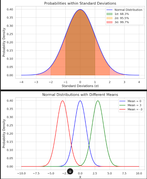
In a normal distribution, the probabilities for data points within 1, 2, and 3 standard deviations from the mean follow the 68-95-99.7 rule:

Graph: Probabilities within standard deviations in a normal distribution.
The mean (μ) determines the center of the normal distribution. Here’s a visualization of three normal distributions with the same standard deviation but different means:

Graph: Normal distributions with varying means.
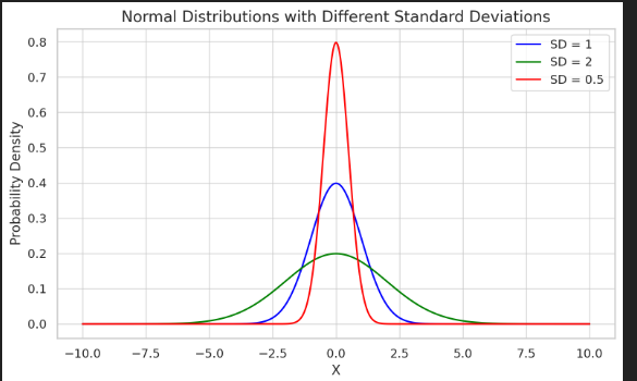
The standard deviation (σ) reflects how spread out the data is. Larger standard deviations result in wider distributions, while smaller ones produce narrower distributions.

Graph: Normal distributions with varying standard deviations.
A practical example of normal distribution is the age of Nobel Prize winners at the time they received the prize. Here’s a histogram fitted with a normal distribution curve:

Graph: Age distribution of Nobel Prize winners.
The normal distribution is a powerful tool for understanding real-world data. By mastering its concepts, you can apply well-known statistical techniques to analyze and interpret data effectively.