Table of Contents
ToggleData analytics is a vital component of modern businesses and research. Python, with its powerful libraries like Pandas, has become a go-to tool for data analysts and scientists. In this blog, we will delve into one of the most powerful and versatile features of Pandas: the GroupBy operation. GroupBy is a fundamental tool for data aggregation, transformation, and exploration. We will explore the magic of GroupBy in Pandas and how it can help you gain valuable insights from your data.
GroupBy in Pandas is similar to the SQL GROUP BY statement. It allows you to group data based on one or more columns, enabling you to perform operations on these groups separately. This functionality is invaluable when dealing with large datasets, as it simplifies data summarization and analysis.
GroupBy is a fundamental operation in data analysis and is a feature commonly found in data manipulation libraries like Pandas in Python, as well as in database systems like SQL. It allows you to group rows of data based on the values in one or more columns, and then perform various operations within each group.
Here’s a breakdown of how GroupBy works:
Grouping: You start by specifying one or more columns by which you want to group your data. These columns contain categorical data, and rows with the same values in these columns are grouped together. Think of it as if you’re partitioning your dataset into smaller, separate subsets.
Aggregation: Once the data is grouped, you can apply aggregation functions to these groups. Aggregation functions perform calculations on each group separately, such as sum, mean, median, count, etc. The result is a summary statistic or a reduced representation of each group.
Transformation: You can also transform the data within each group. This means applying a function to each group that can modify the data within the group. For instance, you could standardize the values within each group or replace missing data with the group’s mean.
Filtering: GroupBy allows you to filter groups based on some condition. For example, you could filter out groups that don’t meet a certain criteria, like groups with a total sum above a certain threshold.
Iteration: You can iterate over the groups, which is useful if you want to perform custom operations for each group.
GroupBy is an essential tool in data analysis, as it enables you to gain insights from your data by exploring patterns and summarizing information within subgroups. It’s especially useful when dealing with large datasets and is widely used in a variety of domains, including business analysis, scientific research, and machine learnin
First, make sure you have Pandas installed. If not, you can install it using pip:
pip install pandas
Then, import Pandas in your Python script:
import pandas as pd
import pandas as pd
Step 2: Create a DataFrame
with your data. In this example, we’ll use a simple dictionary to create a DataFrame:
data = {
    'Category': ['A', 'B', 'A', 'B', 'A', 'C'],
    'Value': [10, 15, 20, 25, 30, 35]
}

df = pd.DataFrame(data)
Use the groupby method to group the data based on a specific column. In this case, we’ll group the data by the ‘Category’ column:
grouped = df.groupby('Category')
You can apply various operations to the groups. Let’s calculate the sum of the ‘Value’ within each group:
result = grouped['Value'].sum()
The result will contain the sum of ‘Value’ for each unique category in the ‘Category’ column.
print(result)
Category
A    60
B    40
C    35
Name: Value, dtype: int64
This output shows the result of grouping and summing the ‘Value’ column based on the ‘Category’ column. It displays the sum of ‘Value’ for each unique category in the ‘Category’ column. In this example:
The sum of ‘Value’ for category ‘A’ is 60.
The sum of ‘Value’ for category ‘B’ is 40.
The sum of ‘Value’ for category ‘C’ is 35.
This is a simple illustration of how the GroupBy operation works in Pandas, allowing you to perform aggregation operations on groups within your dataset.

import pandas as pd

# Load the data from the Excel file
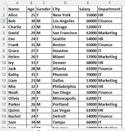
df = pd.read_excel('E:\DATA ANALYTICS\DATASET.xlsx')  # Replace 'sample_data.xlsx' with the actual filename

print(df)
This line of Python code is using the Pandas library to read data from an Excel file named ‘DATASET.xlsx’ located at the file path ‘E:/DATA ANALYTICS/’.
Here’s a breakdown of the line:
This is a variable name used to store the data that will be read from the Excel file. You can choose any valid variable name you prefer.
This is an alias for the Pandas library. Pandas is a popular data manipulation library in Python.
This is a Pandas function that reads data from an Excel file.
‘E:/DATA ANALYTICS/DATASET.xlsx’: This is the file path to the Excel file you want to read. In Python, you can use either double backslashes (\\) or a single forward slash (/) to specify the file path. In this case, the file ‘DATASET.xlsx’ is expected to be located in the ‘E:/DATA ANALYTICS/’ directory.
So, when you run this line of code, it will read the data from the Excel file and store it in the variable df, allowing you to work with the data in your Python program using Pandas functions and method
When you run print(df.info()), it will display something like:
mean_Department_salary = df.groupby('Department')['Salary'].mean()
median_Department_salary=df.groupby('Department')['Salary'].median()
std_Department_salary=df.groupby('Department')['Salary'].std()
print(mean_Department_salary)
print(median_Department_salary)
print(std_Department_salary)
In the provided code, you are using Pandas to calculate various statistics related to salaries within different departments of your DataFrame. Let’s break down the code:
These statistics help you understand the distribution of salaries within different departments, providing insights into the central tendency (mean and median) and the variation (standard deviation) in salary data.
mean_gender_salary = df.groupby('Gender')['Salary'].mean()
median_Gender_salary=df.groupby('Gender')['Salary'].median()
std_Gender_salary=df.groupby('Gender')['Salary'].std()
print(mean_gender_salary)
print(median_Gender_salary)
print(std_Gender_salary)
print(df['Age'].max())
print(df['Age'].min())
# Define the bins for age
age_bins = [20, 25, 30, 35, 40]

# Create a new column for the age bins
df['Age_Bin'] = pd.cut(df['Age'], bins=age_bins, labels=['20-25', '26-30', '31-35', '36-40'])
print(df['Age_Bin'])
Mean_Age_salary = df.groupby('Age_Bin')['Salary'].mean()
mode_Age_salary = df.groupby('Age_Bin')['Salary'].median()
print(Mean_Age_salary)
print(mode_Age_salary) 