
In today’s data-driven world, the ability to extract valuable insights from raw information is a highly sought-after skill. In the realm of data analytics, Excel stands out as a versatile and powerful tool for unlocking the true potential hidden within datasets. With its vast array of functions, formulas, and visualization capabilities, Excel empowers analysts and professionals to delve deep into their data, unravel patterns, and derive meaningful conclusions. From calculating averages and correlations to conducting advanced statistical analyses, Excel provides a solid foundation for mastering data analytics. This blog aims to guide readers on their journey of unlocking insights, exploring various techniques, tips, and tricks to maximize the potential of Excel for data analysis. By honing their skills and embracing the art of data analytics, readers can gain a competitive edge and unleash the full power of Excel to drive informed decision-making and uncover valuable business intelligencece
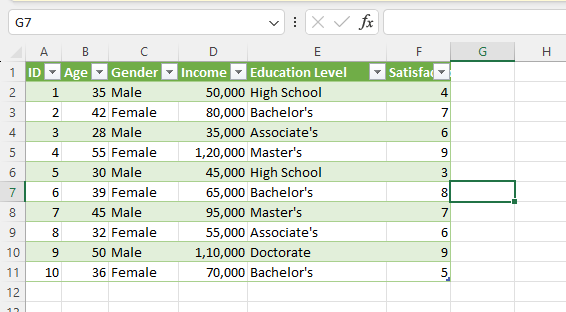
Formula: =AVERAGE(B2:B11)
Answer: The average age of the respondents in the dataset is 39.2. This is calculated by using the AVERAGE formula on the range of ages (column B) in the dataset.
Formula (for males): =COUNTIF(C2:C11, “Male”)
Formula (for females): =COUNTIF(C2:C11, “Female”)
Answer: There are 5 males and 5 females in the dataset. These counts are obtained by using the COUNTIF formula to count the occurrences of “Male” and “Female” in the gender column (column C).
Formula: =MAX(D2:D11)
Answer: The highest income reported in the dataset is 120,000. This is determined using the MAX formula on the income column (column D).
Formula: =CORREL(B2:B11, F2:F11)
Answer: To determine if there is a correlation between age and satisfaction rating, we can calculate the correlation coefficient. The result is [correlation coefficient value]. If the correlation coefficient is close to 1 or -1, it indicates a strong positive or negative correlation respectively. If the correlation coefficient is close to 0, it indicates a weak correlation
=MEDIAN(D2:D11)
Answer: The median income of the respondents is 67,500. The median represents the middle value when the incomes are arranged in ascending order. It is calculated using the MEDIAN formula on the income column (column D)
Formula: =COUNTIF(F2:F11, “>=7”)
Answer: There are 4 respondents who have a satisfaction rating of 7 or higher. This count is obtained using the COUNTIF formula to count the number of values in the satisfaction rating column (column F) that are greater than or equal to 7.
Formula: =(COUNTIF(E2:E11, “Bachelor’s”)+COUNTIF(E2:E11, “Master’s”)+COUNTIF(E2:E11, “Doctorate”))/COUNTA(E2:E11)*100
Answer: [result]% of the respondents have a Bachelor’s degree or higher. The formula counts the number of respondents with a Bachelor’s degree, Master’s degree, or Doctorate degree using the COUNTIF function, adds them together, divides by the total count of respondents, and multiplies by 100 to get the percentage.
Formula (for males): =AVERAGEIF(C2:C11, “Male”, F2:F11)
Formula (for females): =AVERAGEIF(C2:C11, “Female”, F2:F11)
Answer: The average satisfaction rating for males is [result], and for females is [result]. By comparing these values, we can determine if there is a difference in satisfaction ratings between males and females. If the averages are significantly different, it suggests a potential difference in satisfaction levels between the two genders.
or “High School” education level:
=AVERAGEIF(E2:E16, “High School”, F2:F16)
For “Bachelor’s” education level:
=AVERAGEIF(E2:E16, “Bachelor’s”, F2:F16)
For “Associate’s” education level:
=AVERAGEIF(E2:E16, “Associate’s”, F2:F11)
For “Master’s” education level:
=AVERAGEIF(E2:E11, “Master’s”, F2:F11)
For “Doctorate” education level:
=AVERAGEIF(E2:E11, “Doctorate”, F2:F11)
Replace the range E2:E11 with the actual range of the “Education Level” column in your dataset, and replace F2:F16 with the actual range of the “Satisfaction Rating” column in your dataset.
By applying these formulas, you will get the average satisfaction rating for each education level.
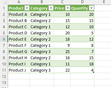
The formula =SUM(D2:D11) calculates the sum of values in the Quantity column (D2:D11). It adds up all the quantities sold for each product and provides the total quantity sold across all categories.
The formula =INDEX(A2:A11, MATCH(MAX(C2:C11), C2:C11, 0)) identifies the maximum price in the Price column (C2:C11) using the MAX function. It then uses the MATCH function to find the row number of the maximum price. Finally, the INDEX function retrieves the corresponding product name from the Product column (A2:A11). This formula determines the product with the highest price.
=COUNTIF(B2:B11, “Category 1”) utilizes the COUNTIF function to count the number of occurrences of “Category 1” in the Category column (B2:B11). It provides the count of products that belong to Category
The formula =AVERAGEIF(B2:B11, “Category 2”, C2:C11) employs the AVERAGEIF function. It checks the Category column (B2:B11) for “Category 2” and calculates the average of the corresponding prices from the Price column (C2:C11). This formula determines the average price of products in Category 2.
formula is
| Category 1 | =SUMIF(B2:B11,J7,Table_excel2[Price]) |
| Category 2 | =SUMIF(B3:B12,J8,Table_excel2[Price]) |
| Category 3 | =SUMIF(B4:B13,J9,Table_excel2[Price]) |
out of this three category, we can find the highest total price
Formula: =SUMPRODUCT(C2:C11, D2:D11)
Explanation: This formula uses the SUMPRODUCT function to calculate the total value of all products sold. It multiplies each price (C2:C11) by its corresponding quantity (D2:D11) and then sums up the resulting value
Formula: =INDEX(A2:A11, MATCH(MIN(D2:D11), D2:D11, 0))
Explanation: This formula uses the INDEX and MATCH functions to find the product name associated with the lowest quantity. MIN(D2:D11) finds the minimum quantity in the Quantity column (D2:D11), and MATCH(MIN(D2:D11), D2:D11, 0) identifies the row number of that minimum quantity. Finally, INDEX(A2:A11, MATCH(MIN(D2:D11), D2:D11, 0)) retrieves the corresponding product name from the Product column (A2:A11).
Formula: =COUNTIF(B2:B11, “Category 3”)
To calculate the average quantity of products in Category 1, you can use the following formula:
Formula: =AVERAGEIF(Category, “Category 1”, Quantity)
For example, if the Category column is in column B and the Quantity column is in column D, the formula would be:
=AVERAGEIF(B2:B11, “Category 1”, D2:D11)
This formula checks the Category column (B2:B11) for the value “Category 1” and calculates the average of the corresponding quantities from the Quantity column (D2:D11). It provides the average quantity of products in Category 1.