
AI के युग में Critical Thinking: 2026 में इंसान की सबसे ज़रूरी स्किल
परिचय (Introduction) AI युग, 2026 और सोचने की असली ताकत वर्ष 2026 तक Artificial Intelligence केवल एक तकनीक नहीं रह […]
AI Course 2026 – Free AI Tools & Workflows Guide (Beginner to Advanced) | Vista Academy
SECTION 1: Introduction – Why AI Matters in 2026 Artificial Intelligence अब भविष्य नहीं, वर्तमान है Artificial Intelligence (AI) आज […]
Hypothesis meaning in Hindi with example
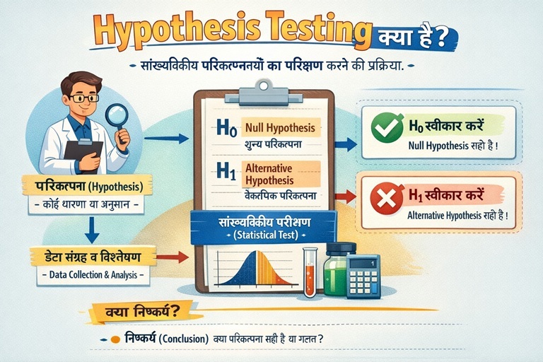
Hypothesis Testing क्या है? (परिकल्पना परीक्षण) Statistics & Data Analytics का सबसे ज़रूरी concept आज के समय में हम हर […]
Emotional Intelligence क्या है? | AI के युग में Emotional Intelligence क्यों सबसे ज़रूरी Skill बन गई है (2025 Guide)

1. Emotional Intelligence (EI) का अर्थ क्या है? What is Emotional Intelligence? Emotional Intelligence (EI) का मतलब है अपनी और […]
कंप्यूटर मेमोरी वास्तव में कैसे काम करती है? | 0 और 1 से पूरी डिजिटल दुनिया कैसे बनती है
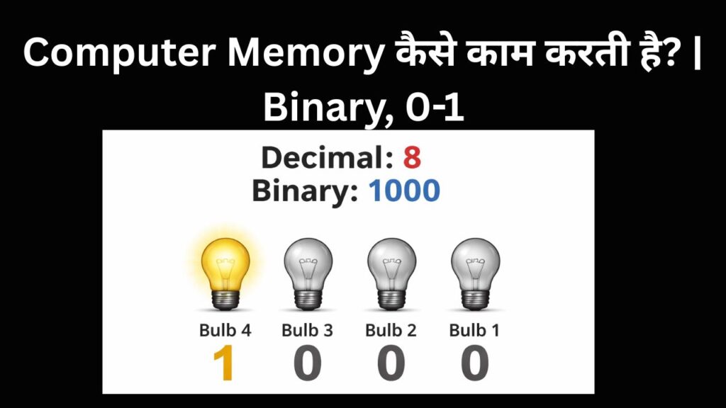
💾 कंप्यूटर मेमोरी कैसे काम करती है? Computer Memory in Hindi: Binary (0 और 1), Bit–Byte, RAM और Digital Storage […]
Data Analyst Internship kaise milegi? (2025 Complete Roadmap – Fresher ke liye)

Data Analyst Internship kaise milegi? 2025 Complete Roadmap for Freshers अगर आप एक फ्रेशर हैं और आपके पास अभी कोई […]
भारत में Data Analyst कैसे बनें: ज़रूरी स्किल्स, सरकारी और प्राइवेट नौकरी का पूरा रोडमैप (2026)
VA भारत में Data Analyst कैसे बनें: ज़रूरी स्किल्स, सरकारी व प्राइवेट नौकरी का रोडमैप (2026) कव्हर: SQL, Python, Power […]
SQL Joins in Hindi | INNER, LEFT, RIGHT, FULL Join Explained

Section 1 • Quick Concept SQL Joins — आसान परिचय (INNER, LEFT, RIGHT, FULL) ⏱ 3–5 min यह section beginners […]
देहरादून ISBT बस टाइम टेबल 2026 | Delhi, Haridwar, Fare & Route
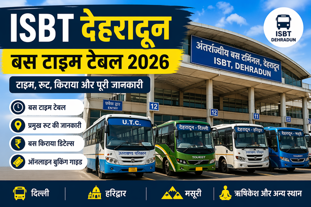
देहरादून ISBT (बस अड्डा): बस टाइम टेबल, रूट, किराया, और ऑनलाइन बुकिंग की संपूर्ण गाइड उत्तराखंड की राजधानी देहरादून केवल […]
AI, ML, DL, और डेटा साइंस Full Form A to Z: भविष्य की टेक्नोलॉजी का महाकोष

🧠 AI, ML, DL, और डेटा साइंस — Full Form A to Z: भविष्य की टेक्नोलॉजी का महाकोष एक अंतिम […]
डेटा एनालिटिक्स करियर रोडमैप 2026: कौशल, नौकरियाँ और भविष्य के ट्रेंड्स (हिंदी)
डेटा एनालिटिक्स करियर रोडमैप 2026: कौशल, नौकरियाँ, और भविष्य के ट्रेंड्स (इंटरैक्टिव गाइड) AI और क्लाउड तकनीकों द्वारा संचालित, डेटा […]
How to Build a Student Performance Dashboard Using Data Analytics (Beginner to Intermediate Guide)
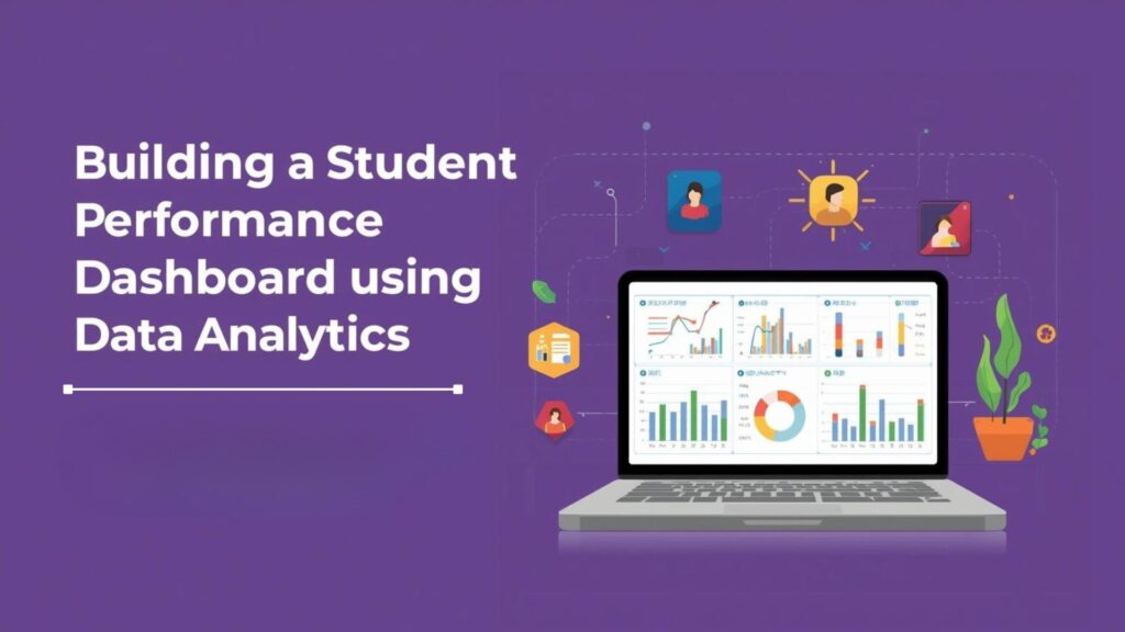
Student Performance Data Analytics Project Interactive online dashboard using a real school dataset — beginner-friendly guide and practice project for […]