Common data problems are simple to solve using Power Query. Most of our valuable time is frequently consumed by tedious manual procedures like cut and paste labour, column merging, and filtering. These operations are greatly simplified with the Power Query tool.
Table of Contents
Toggle
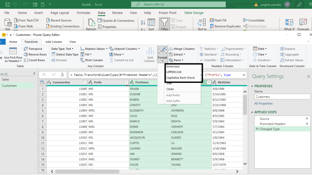
An application for preparing and transforming data is called Power Query. With Power Query, you may perform transformations to data obtained from sources using a Power Query Editor and a graphical user interface. You may import data from a variety of sources, clean it up, convert it, and then reshape it to suit your needs using Power Query, a business intelligence tool provided by Microsoft Excel. This allows you to create a query just once and reuse it at a later time by simply refreshing.
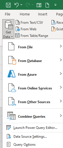
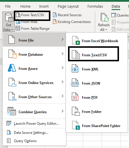
Power Query, as its name suggests, is Excel 2010 and later’s most potent data automation tool. Data may be imported into Excel using Power Query from a variety of external sources, including Excel workbooks, CSV files, text files, and the web, to name a few.
Power Query includes a number of helpful capabilities, including the ability to append data and establish connections across various data sources. The joining of the data sets is what this is known as. The tool also allows us to group and condense data. Without a doubt, it is a very helpful tool.
You may get Power Query for free as an add-in for Excel 2010 and 2013 from Microsoft’s website. You can access the URL here.
When you click the Download button, a dialogue box where you may select the best download option for your OS opens. Your machine will then download Power Query.
Starting with Excel 2016, it is a built-in tool that can be found in the Data Tab’s Get & Transforms Data Section.
Let’s continue and comprehend the Power Query idea.
Data can be imported from a variety of sources.
Excel files (Workbooks), text or CSV files, XML files, and JSON files can all be read from files.
SQL Server, Microsoft Access, and SQL Server Analysis Services are databases.
Excel Tables/Ranges, the Web, Microsoft Query, and OData feeds are some additional sources.
With the use of Power Query, we may change the data after importing it. You can modify data according to your needs with the help of the Power Query Editor.Let’s examine the editor and learn about its various parts.
The Power Query Editor has the following six key sections:
Follow the steps below to learn how to sort a table based on a single column.
We must output the editor’s operations to our Excel sheet after finishing them all. To accomplish this, select Close and Load from the Power Query Editor’s Ribbon menu.
Listed below is a detailed tutorial of importing data from various data sources.
1. Importing Data from a Text File
To import a text file using Power Query, follow these steps:
Click Text/CSV File under the Data tab.
After choosing “Text/CSV file,” a new “Import data” dialogue box appears.
Click Import after choosing the text file you want to import.
When a dialogue box is opened, a preview of the data inside is displayed.
To import the data, click Load at the very end.
You can use Power Query to import from CSV files by following the steps below:
You can import various data sources from the Excel workbook by following these steps:
Select the Get data command after clicking the Data tab. When you click it, a drop-down menu appears. We can import our data using a variety of options from the drop-down menu. We choose “From File” and then “From Workbook” to import data from an Excel workbook.
Excel displays a dialogue box to aid in selecting and navigating the workbook.
Once we have found the worksheet, we can click on it and choose “Open” from the menu.
The navigation dialogue box appears as a result. You can access a number of data sources from the navigation dialogue box.
Step 1: Fill the Power Query Editor with the necessary data. To achieve this, choose the appropriate data source from the Excel Data tab’s Get & Transform Data section. This will launch the Editor, which enables data editing.
Step 2: After clicking the column name, select the “Transform” tab to get a range of possibilities. When you select the option to format text, a drop-down menu with the option to alter text in “UPPERCASE” will appear.
Finally, on selecting the UPPERCASE edit option, all the text in the given column will be converted to uppercase.
Step 1: Fill the Power Query Editor with the necessary data. Choose the appropriate data source from the Get & Transform Data section of the Excel data tab to accomplish this. This will launch the Editor, which enables data editing.
Step 2: Click the name of the column, then select the “Transform” tab to see a range of options. When you select the text formatting option, a drop-down menu with the text editing choice “LOWERCASE” will appear.
Step 1: Fill the Power Query Editor with the necessary data. Choose the appropriate data source from the Get & Transform Data section of the Excel data tab to accomplish this. The Power Query Editor will then be displayed, allowing us to alter the data.
Step 2: Click on the column name and then choose the “Transform” tab, which will present you with a number of options, to eliminate all extra white spaces from the data. When you select the “Format” option, a drop-down menu with the “Trim” text editing option will appear.
Finally, on selecting the Trim edit option, all the extra white spaces in the given column will be removed.
Step 1: Fill the Power Query Editor with the necessary data. Choose the appropriate data source from the Get & Transform Data section of the Excel data tab to accomplish this. This will launch the Editor, which enables data editing.
Step 2: Select the “Transform” tab, then the “Split column” option, to divide the column using a delimiter from the data. A drop-down menu with the option to divide the data by delimiter will appear as a result.