
Table of Contents
ToggleNow we will explain how we found the slope and intercept of our function:
The formula for the linear function is: f(x) = 2x + 80
The image below points to the Slope — which indicates how steep the line is, and the Intercept — which is the value of y when x = 0 (the point where the diagonal line crosses the vertical axis). The red line is the continuation of the blue line from the previous page.
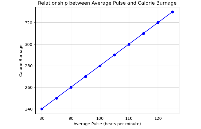
Look at the line. What happens to calorie burnage if the average pulse increases from 80 to 90?
The slope is defined as how much calorie burnage increases, if the average pulse increases by one. It tells us how “steep” the diagonal line is.
We can find the slope by using the proportional difference of two points from the graph.
If the average pulse is 80, the calorie burnage is 240.
If the average pulse is 90, the calorie burnage is 260.
We see that if the average pulse increases by 10, the calorie burnage increases by 20.
Slope = 20 / 10 = 2
The slope is 2.
Mathematically, the slope is defined as:
Slope = (f(x2) – f(x1)) / (x2 – x1)
Where:
Now, calculating the slope:
Slope = (260 – 240) / (90 – 80) = 2
Be consistent to define the observations in the correct order! If not, the prediction will not be correct!
In this tutorial, we will learn how to use Python to calculate the slope and intercept of a linear function, which helps us predict calorie burnage based on average pulse. Understanding the slope and intercept is essential for making predictions using linear regression.
The slope of a line is an indicator of how steep the line is. In the context of calorie burnage, it tells us how much the calorie burnage increases when the average pulse increases by one.
def slope(x1, y1, x2, y2):
  s = (y2 - y1) / (x2 - x1)
  return s

print(slope(80, 240, 90, 260))
In this example, the slope is calculated between two points (80, 240) and (90, 260), where the average pulse increases from 80 to 90, and the calorie burnage increases from 240 to 260. The result of this calculation is the slope of the line.
The intercept is the point where the line crosses the y-axis. It represents the value of the dependent variable (calorie burnage) when the independent variable (average pulse) is zero. Although the intercept may not always have practical significance, it is necessary for completing the linear function to make accurate predictions.
In our case, when the average pulse is zero, the calorie burnage is 80, so the intercept is 80. While a pulse of zero doesn’t make sense biologically, the intercept is required for the mathematical function to work correctly.
We can calculate the slope and intercept using the np.polyfit() function from the NumPy library. This function fits a polynomial of a given degree to the data. For linear functions, the degree is 1.
import pandas as pd
import numpy as np

health_data = pd.read_csv("data.csv", header=0, sep=",")

x = health_data["Average_Pulse"]
y = health_data["Calorie_Burnage"]
slope_intercept = np.polyfit(x, y, 1)

print(slope_intercept)
This code reads data from a CSV file, isolates the Average_Pulse and Calorie_Burnage columns, and calculates the slope and intercept. The result is an array containing the slope and intercept.
Once we have the slope and intercept, we can use the linear function to predict the calorie burnage for a given average pulse. For instance, if the average pulse is 135, we can substitute it into the formula:
f(135) = 2 * 135 + 80 = 350If the average pulse is 135, the predicted calorie burnage is 350.
Now, let’s define the mathematical function in Python using the calculated slope and intercept:
def my_function(x):
  return 2 * x + 80

print(my_function(135))
This Python function returns the calorie burnage for any given average pulse based on the formula f(x) = 2 * x + 80.
Finally, we can plot the data using the matplotlib library to visualize the relationship between average pulse and calorie burnage:
import matplotlib.pyplot as plt

health_data.plot(x='Average_Pulse', y='Calorie_Burnage', kind='line')
plt.ylim(ymin=0, ymax=400)
plt.xlim(xmin=0, xmax=150)

plt.show()
This code plots a line graph showing the relationship between Average_Pulse and Calorie_Burnage, with the y-axis ranging from 0 to 400 and the x-axis from 0 to 150.